
Policy Gradient - Actor-Critic
This page picks up where the REINFORCE notes left off, following Lecture 6: Actor-Critic from CS 285. We move from a Monte Carlo critic to a bootstrapped one and build up to generalized advantage estimation. We will still rely on Homework 2 to show some results.
Preamble
In the REINFORCE notes we used a value network $V_\varphi$ as a baseline, fit to Monte Carlo returns. It reduced variance, but it never really earned the name "critic". Here we make it one. The key idea is bootstrapping: letting the value function estimate the future instead of always rolling it out.
What makes a critic
It is worth being precise about terminology, because it tripped me up. In the REINFORCE notes the value network was used purely as a baseline: we subtracted it from the Monte Carlo return, and that was it. The return itself came entirely from real, sampled rewards.
Sutton & Barto are strict about this (§13.5, p. 331): a method is only actor-critic if the value function is used to bootstrap, meaning the update target depends on the value estimate of a later state. REINFORCE-with-baseline does not bootstrap, so despite having a value network, it is not actor-critic. The value function there is just a baseline.
The TD error
Bootstrapping shows up through the temporal-difference (TD) error. To see where it comes from, start from the definition of the value function as an expectation. The Bellman expectation equation says the value of a state is the expected immediate reward plus the discounted value of wherever we land next:
$$V^{\pi}(s_t) = \mathbb{E}_{a_t \sim \pi,\, s_{t+1}}\big[\, r(s_t, a_t) + \gamma\, V^{\pi}(s_{t+1}) \,\big]$$The TD error is just the single-sample residual of this equation, the gap between the two sides for one observed transition:
$$\delta_t = r_t + \gamma\, V_\varphi(s_{t+1}) - V_\varphi(s_t)$$Two things make this useful:
- If $V_\varphi$ were exactly right, $\delta_t$ would average to zero. When it is off, $\delta_t$ tells us by how much, and that is the signal we use to train the critic.
- $\delta_t$ is also a one-sample estimate of the advantage: its average is $\mathbb{E}[\delta_t] = Q^{\pi} - V^{\pi} = A^{\pi}(s_t, a_t)$. So $\delta_t$ does two jobs at once, it trains the critic and it is the advantage for the actor.
A basic actor-critic algorithm
Now we know about the TD error, we can design a simple critic. Use $\delta_t$ as the advantage for the actor, and train the critic on the bootstrapped target $y = r + \gamma V_\varphi(s')$.
It is the same loop as before (generate samples, fit the value model, improve the policy). The only change is that both the critic target and the advantage now bootstrap through $V_\varphi$.
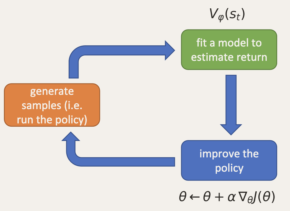
It helps to recap the advantage estimators we have seen so far:
| advantage | bias | variance |
|---|---|---|
| MC reward-to-go (REINFORCE) | none | highest |
| reward-to-go $-\, V_\varphi$ (baseline) | none | lower |
| $r + \gamma V_\varphi(s') - V_\varphi$ (bootstrap) | some, if $V_\varphi$ is imperfect | lowest |
The first two we covered in the REINFORCE notes. The bootstrapped one is the actual actor-critic, and there is bias since $V_\varphi$ is never exactly right.
Generalized advantage estimation
The 1-step TD advantage $\delta_t$ has low variance but is biased, since it entirely depends on $V_\varphi$ being correct. At the other extreme, the Monte Carlo advantage uses only real rewards (no bootstrap), so it is unbiased but high variance. These are the two ends of a spectrum.
You can actually slide between them by using an n-step advantage. It takes $n$ real rewards, then bootstraps with $V_\varphi$ for the rest. You are effectively moving the cost-to-go estimate further down the known part of the trajectory:
$$\hat{A}_n(s_t, a_t) = \sum_{t'=t}^{t+n-1} \gamma^{t'-t} r(s_{t'}, a_{t'}) + \gamma^n V_\varphi(s_{t+n}) - V_\varphi(s_t)$$$n=1$ gives back $\delta_t$ (full bootstrap), and $n$ large recovers the Monte Carlo advantage (no bootstrap). The further out you bootstrap, the less you lean on $V_\varphi$ so the less bias, but the more accumulated reward noise you carry so the more variance. From what I understand choosing $n > 1$ often works better than either extreme.
The intuition is that the further into the future you look, the more the trajectories fan out and the noisier the return gets. You want to cut the rollout off before the variance blows up and let $V_\varphi$ estimate the tail.
Rather than commit to a single $n$, GAE takes an exponentially weighted average of all the $n$-step advantages, with decay $\lambda \in [0, 1]$:
$$\hat{A}^{\text{GAE}}_t = (1 - \lambda) \sum_{n=1}^{\infty} \lambda^{n-1}\, \hat{A}_n(s_t, a_t)$$After the $V_\varphi$ terms telescope, this collapses to a clean sum of TD errors:
$$\hat{A}^{\text{GAE}}_t = \sum_{l=0}^{\infty} (\gamma\lambda)^{l}\, \delta_{t+l}$$computed cheaply with the backward recursion
$$\hat{A}^{\text{GAE}}_t = \delta_t + \gamma\lambda\, \hat{A}^{\text{GAE}}_{t+1}.$$In code it is just that recursion, swept backwards over the batch. The same function picks between the plain baseline (Monte Carlo advantage) and GAE on whether gae_lambda is set:
values = ptu.to_numpy(self.critic.forward(ptu.from_numpy(obs)).squeeze(-1))

if self.gae_lambda is None:
    advantages = q_values - values
else:
    batch_size = obs.shape[0]

    values_ext = np.append(values, [0])
    advantages = np.zeros(batch_size + 1)

    for i in reversed(range(batch_size)):

        if terminals[i]:
            advantages[i] = rewards[i] - values_ext[i]
        else:
            advantages[i] = rewards[i] + self.gamma * values_ext[i+1] - values_ext[i] + self.gae_lambda * self.gamma * advantages[i+1]

    # remove dummy advantage
    advantages = advantages[:-1]
- $\lambda = 0$: only the $l=0$ term survives, so $\hat{A}_t = \delta_t = r_t + \gamma V_\varphi(s_{t+1}) - V_\varphi(s_t)$. This is the pure 1-step TD advantage: maximum bootstrapping, lowest variance, most bias.
- $\lambda = 1$: the $V_\varphi$ terms telescope and we are left with $\hat{A}_t = \sum_{l=0}^{\infty} \gamma^{l} r_{t+l} - V_\varphi(s_t)$, the Monte Carlo reward-to-go minus the baseline. No bootstrapping: unbiased, highest variance.
So $\lambda$ is the bias-variance knob between full bootstrap ($\lambda=0$) and pure Monte Carlo ($\lambda=1$). The full derivation is in section 3 of the CS285 notes.
The algorithm is the batch actor-critic from above, with the advantage swapped for the GAE estimate:
Two critic targets
The algorithm above shows a simple bootstrapped target for the critic. The homework, though, asks the critic to be fit on a Monte Carlo return instead. On this page we will actually compare 2 different critics:
- MC critic. Fit $V_\varphi(s_t)$ to the actual discounted reward-to-go. No bootstrapping in the critic at all.
- GAE critic. Fit $V_\varphi(s_t)$ to the bootstrapped λ-return, which we get straight from the advantage:
So the value target is just the advantage plus the current value estimate. With $\lambda = 0$ it is the 1-step TD(0) target $r + \gamma V_\varphi(s')$ (which matches the algorithm above). With $\lambda = 1$ it telescopes to the full Monte Carlo return, which is exactly the MC critic target, so at $\lambda = 1$ the two critics should match in theory. The GAE critic is what the gae_critic_target flag turns on in the code.
So we have two experiments to run: the same $\lambda$ sweep, once with the MC critic and once with the GAE critic.
Fitting the critic
Before moving on to the results, there were two things about training the critic that confused me, so I wanted to point them out and expand on them.
First, does the $V$ cancel? The critic loss is $\|V^{\text{target}}(s_t) - V_\varphi(s_t)\|^2$, and the residual is exactly $\hat{A}^{\text{GAE}}_t$, so it looks like the $V$ cancels and the loss is just the squared advantage. It does not, because the target is detached: it is a fixed constant, while the $V_\varphi(s_t)$ being trained is the live network. So the gradient is real and pushes the critic toward the target. In the code the detach lives in the numpy helper that pulls the value estimate out before the target is built:
def to_numpy(tensor):
    return tensor.to('cpu').detach().numpy()
This is the semi-gradient trick (I am starting to see it everywhere in RL) and it makes sense. It is needed whenever the target is built from the function you are training (any kind of bootstrapping). Take a bootstrapped target $y = r + \gamma V_\varphi(s')$. The honest gradient of the loss $L = \tfrac{1}{2}\big(y - V_\varphi(s)\big)^2$ is
$$\nabla_\varphi L = -\big(y - V_\varphi(s)\big)\,\big(\nabla_\varphi V_\varphi(s) - \gamma\, \nabla_\varphi V_\varphi(s')\big),$$and the semi-gradient just drops the second term, the one that flows through the target:
$$\nabla_\varphi^{\text{semi}} L = -\big(y - V_\varphi(s)\big)\, \nabla_\varphi V_\varphi(s).$$Keeping the dropped term would be cheating. Look at the full loss $\tfrac{1}{2}\big(r + \gamma V_\varphi(s') - V_\varphi(s)\big)^2$: you can shrink it two ways. Either push $V_\varphi(s)$ up to meet the target (real learning), or push $V_\varphi(s')$ down so the target drops to meet the prediction. That second route just lowers the next-state value to balance the equation, learning nothing real. For our advantage formulation the loss would just be $\tfrac{1}{2}\hat{A}_t^2$, so the network would just drive every advantage to zero. Detaching the target prevents this and forces the network to actually fit it.
The second concern I had was whether the critic error going to zero forces the advantage to zero too. It does not, and the reason is the squared-error fit, not the detaching. First, note that the residual is just the advantage again: the target is $\hat{A}_t + V_\varphi(s_t)$, so the target minus the prediction is $\hat{A}_t$ (the $V_\varphi$ cancels). Now, minimizing $\big(V^{\text{target}}(s_t) - V_\varphi(s_t)\big)^2$ lands $V_\varphi(s_t)$ on the average target at each state, so the average residual is zero. That means the average advantage per state goes to zero, not the individual ones, which stay positive for good actions and negative for bad ones. This is actually exactlywhat we want. Detaching matters for a different reason: without it the optimizer would cheat and drive every residual to zero, not just the average.
Setup
To see the bias-variance knob in action, I swept $\lambda \in \{0, 0.95, 0.98, 0.99, 1\}$ on LunarLander-v2 with noisy actions. As described above, I run this sweep twice, once with the MC critic and once with the GAE critic. Everything else is shared and fixed:
- Environment: LunarLander-v2 with noisy actions, episodes up to 1000 steps.
- Policy and critic: 3-layer MLP, 128 units per layer.
- Discount: $\gamma = 0.99$.
- Batch: 2000 environment steps per iteration, 2000 for eval.
- Learning rate: $10^{-3}$.
- Iterations: 200.
- Swept: the GAE $\lambda$ over the five values above.
uv run src/scripts/run.py --env_name LunarLander-v2 --ep_len 1000 --discount 0.99 \
  -n 200 -b 2000 -eb 2000 -l 3 -s 128 -lr 0.001 --use_reward_to_go --use_baseline \
  --gae_lambda <lambda> --exp_name lunar_lander_lambda<lambda>
LunarLander is noisy and sensitive to the seed, so each curve below is the best of a few seeds, which is also how the homework asks you to report.
MC critic results
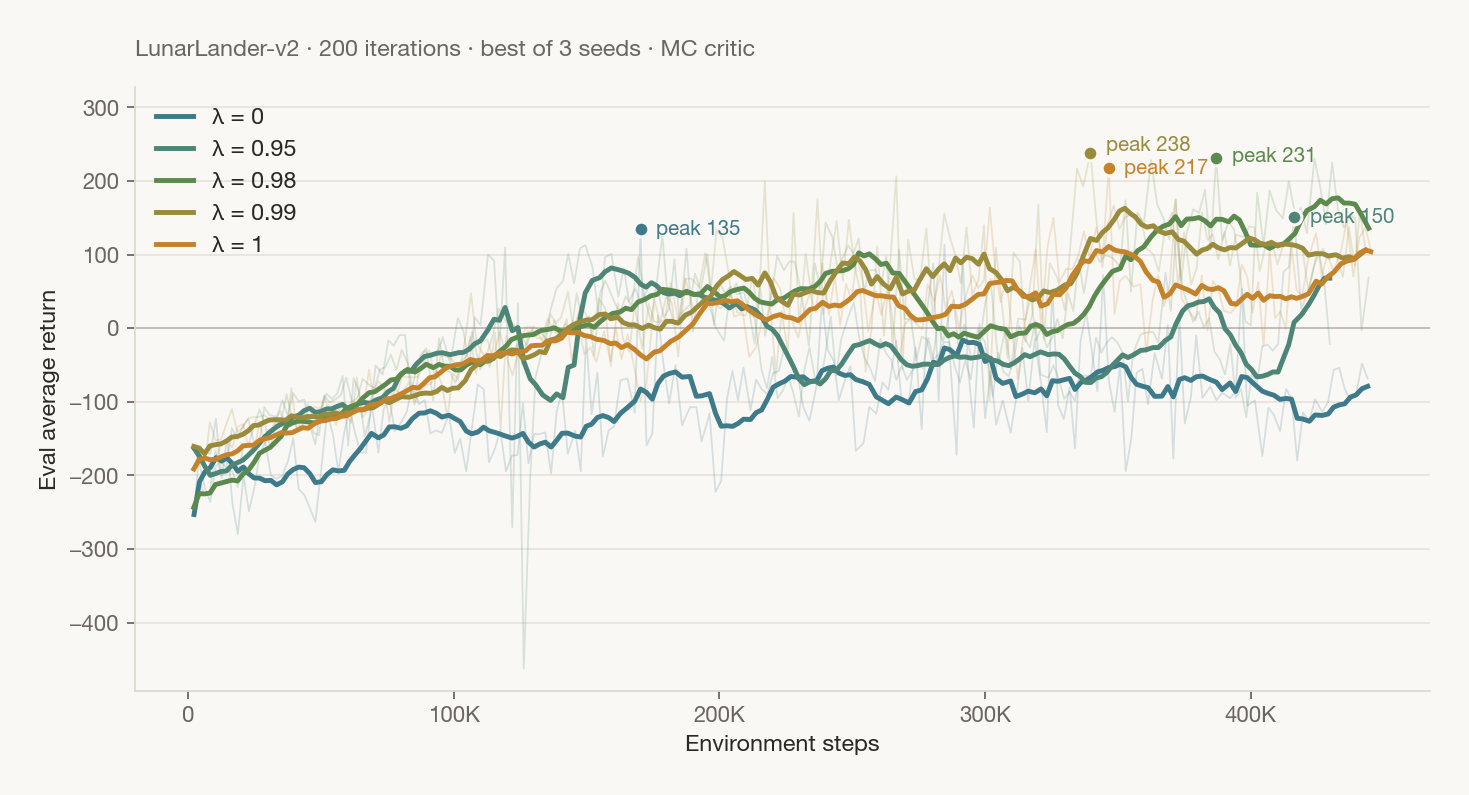
$\lambda = 0$ is the pure 1-step TD advantage, $\delta_t = r_t + \gamma V_\varphi(s_{t+1}) - V_\varphi(s_t)$, and is clearly the worst here. I think the reason pure bootstrapping struggles is that the advantage leans entirely on the critic:
- Early in training $V_\varphi$ is essentially random, so the advantage is dominated by critic error rather than real signal. The bias is effectively very high in that case.
- Even later, $V_\varphi$ is only a neural-network approximation of a tough value problem (long episodes, reward concentrated at the landing), so some error always remains and keeps biasing the 1-step advantage.
Higher $\lambda$ mixes in real returns, which do not rely as much on the critic being right. That is probably why even $\lambda = 0.95$ solves the task while $\lambda = 0$ stalls. Among the $\lambda \ge 0.95$ runs the differences look like seed noise to me, so I would not read too much into the ordering.
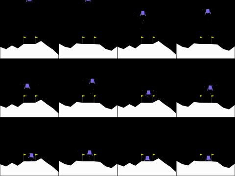
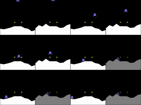
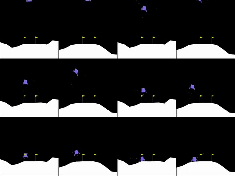
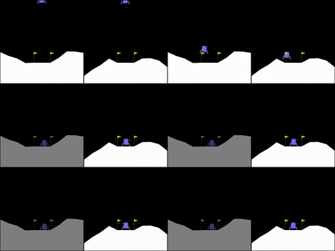
Here is what the best policy for each $\lambda$ actually does at the end of training:
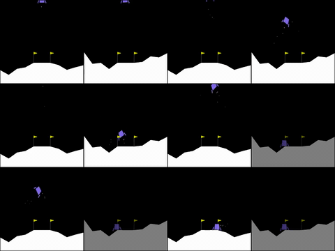
peak 135
peak 150
peak 231
peak 238
peak 217
GAE critic results
Now the second sweep. Same $\lambda$ values, but the critic is trained on the bootstrapped λ-return instead of Monte Carlo reward-to-go (the -gct flag).
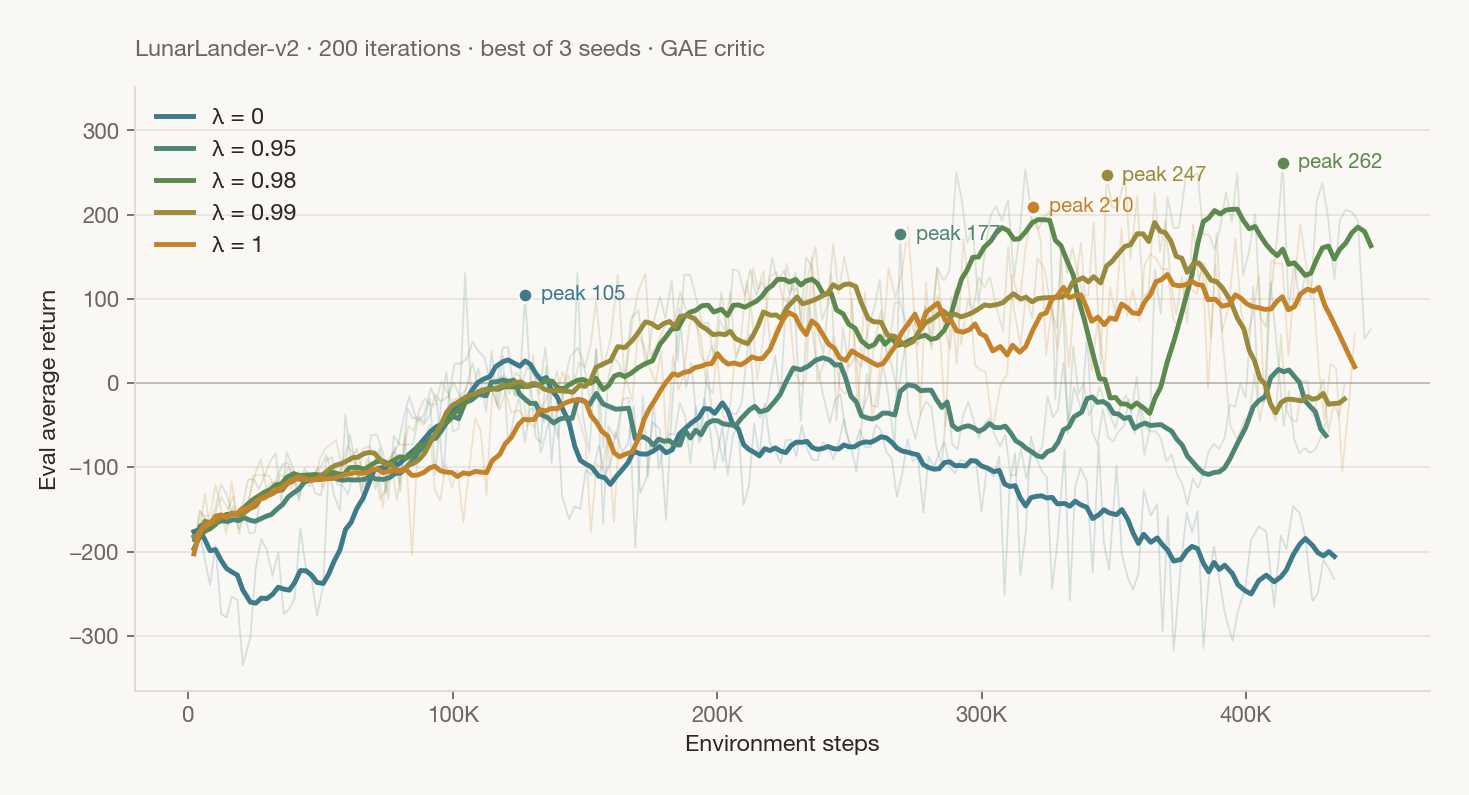
Putting the two critics side by side (best-of-3 peak per λ):
| λ | MC critic | GAE critic |
|---|---|---|
| 0 | 135 | 105 |
| 0.95 | 150 | 177 |
| 0.98 | 231 | 262 |
| 0.99 | 238 | 247 |
| 1 | 217 | 210 |
Three things stand out.
The high-λ runs ($\lambda \ge 0.95$) do a little better than the MC critic. I think this makes sense. Bootstrapping lowers the critic's variance, and at high λ the advantage still has enough real signal that the added bias stays small.
$\lambda = 1$ almost matches between the two critics (210 vs 217), which is the consistency check from earlier: at $\lambda = 1$ the GAE target telescopes to the Monte Carlo return, so the two are the same target in theory.
$\lambda = 0$ is the interesting one. Here the GAE critic (105) does worse than the MC critic (135). I think this is related to the reward propagation issue mentioned earlier. The MC critic learns the full return, so it knows the landing outcome at every state right away. The GAE critic at $\lambda = 0$ only uses a 1-step target $r + \gamma V_\varphi(s')$, so the landing reward has to walk back to the start one state per update. On LunarLander, which has long episodes, this seems to lead to poor performance: you are stuck with a wrong critic for a while (high bias) and it learns very slowly.
Here are the best GAE-critic policies at the end of training:
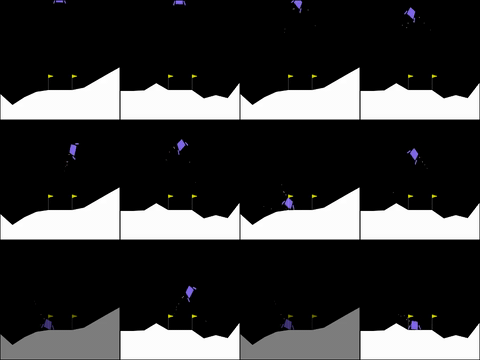
peak 105
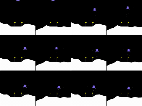
peak 177
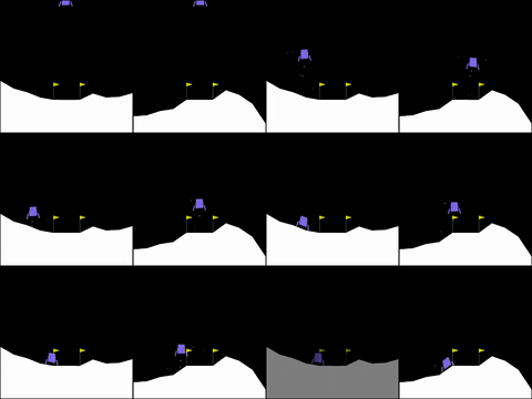
peak 262
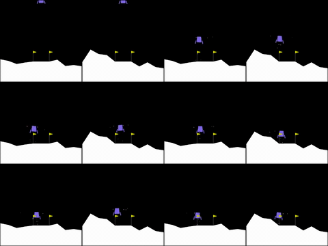
peak 247
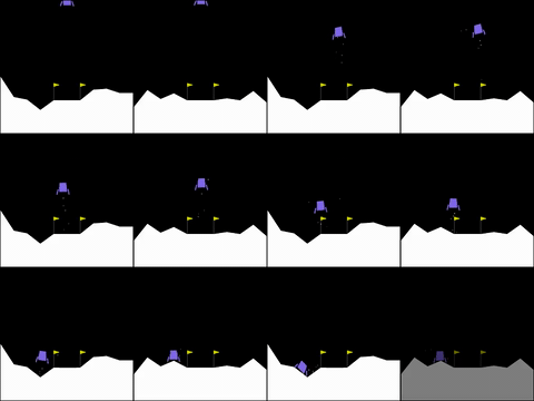
peak 210
Conclusion
That is it for the policy gradient with a critic. I feel this was a great way to lay the foundation before moving on to more advanced methods. I especially like the elegance of the GAE formulation: a single "pareto knob" $\lambda$ that controls the bias-variance tradeoff.
Everything so far has been on-policy. Next we will look at how to do off-policy learning, and all the tricks needed to make it work. On to Q-learning!
References
- CS 285 Deep RL, UC Berkeley. Lecture 6: Actor-Critic. Spring 2026. rail.eecs.berkeley.edu/deeprlcourse.
- CS 285 Deep RL, UC Berkeley. HW2: Policy Gradients (PDF) and the section 3 notes on GAE.
- Sutton & Barto. Reinforcement Learning: An Introduction, 2nd ed. PDF. §13.5 Actor-Critic Methods (p. 331) draws the baseline-vs-critic line.
Terminal reward
If you read all the way through, you have earned a classic. Run ./run_me.sh in the terminal on the homepage.