Behavioral Cloning

Four Push-T rollout episodes. The agent (blue dot) pushes the grey T-block toward the green goal pose.

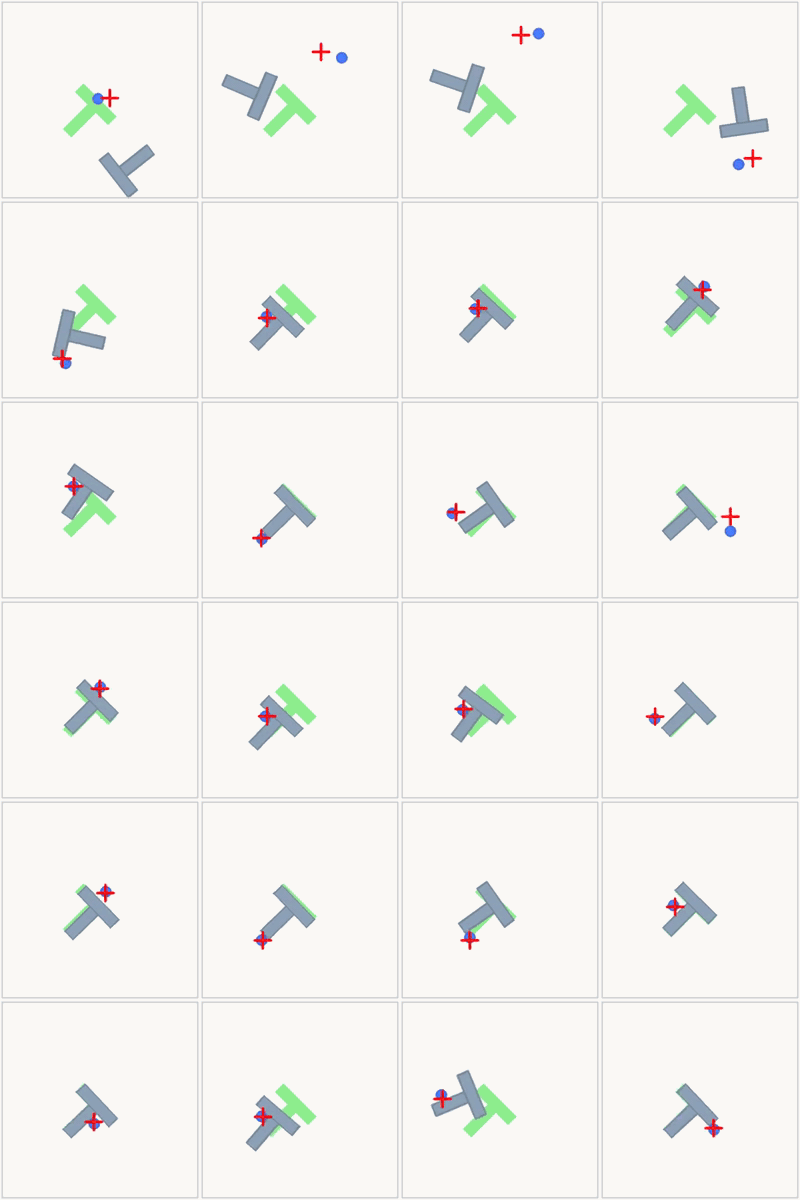
Push-T is a 2-D manipulation benchmark where a robot end-effector must push a T-shaped block into a fixed goal configuration. The state $s \in \mathbb{R}^5$ encodes the agent position $(x_a, y_a)$ and the block pose $(x_b, y_b, \theta_b)$; the action $a \in \mathbb{R}^2$ is a target 2-D position for the end-effector. The dataset contains ~25,000 human-teleoperated demonstrations stored as a Zarr replay buffer.

The reward at evaluation is the overlap between the current block footprint and the goal region, a number in $[0, 1]$.

Behavioral cloning can be seen as a simple supervised regression problem. Given a dataset of expert state-action pairs $\mathcal{D} = \{(s_i, a_i)\}_{i=1}^N$ collected under expert policy $\pi^*$, the goal is to maximize the likelihood of the learned policy to behave similarly to the expert. It is effectively an MLE problem:

or more generally, minimizing a loss $\ell$ over the dataset:

We evaluate two approaches. Since the action space is continuous, the simplest choice is an MSE cost. We also consider flow matching, a generative diffusion-like approach. Both are evaluated and discussed in the results section.

The principal problem with BC is that training is done on the expert's state distribution $p_{\text{train}}$, while at test time the policy rolls out under its own distribution $p_{\pi_\theta}$. The moment it deviates slightly, it enters states the expert never visited and the policy won't likely recover.

A small initial deviation (red) steers the policy off the expert manifold. Everything downstream is out-of-distribution; the cloned policy compounds errors rather than recovering.

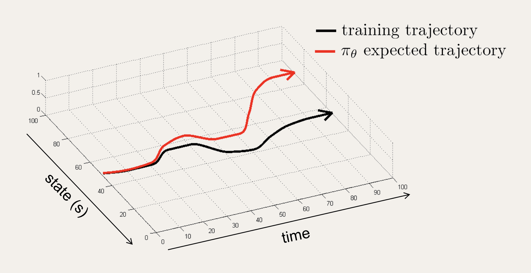
The $O(\epsilon H^2)$ bound

Assume $\mathbb{E}_{s_t \sim p_{\text{train}}}[\pi_\theta(a_t \neq \pi^*(s_t) \mid s_t)] \leq \epsilon$, i.e., for any given training state, the probability that the BC policy disagrees with the expert is at most $\epsilon$.

Over a full trajectory, the total expected number of mistakes is bounded by:

This becomes tight when every mistake causes irreversible distribution shift. A single error sends you into completely out-of-distribution states with no path back to the expert's trajectory. Think of a tightrope, one misstep and you've fallen off entirely.

The cost grows quadratically in horizon $H$. A per-step error rate that looks harmless on short tasks can become very large over longer horizons. This is reminiscent of how small $\epsilon$ errors cause instability in control systems when integrated forward without correction (think open-loop MPC or discretization error accumulation).

DAgger

Like a control system, one fix is to provide feedback to stabilize the system, but at a very low bandwidth where we ask experts to re-label the data for states visited by the policy (some of which might have caused the policy to fail) so the training distribution converges to the policy's own distribution and the bound drops to $O(\epsilon H)$:

Rather than predicting a single action $a_t \in \mathbb{R}^2$ at each step, the policy outputs a chunk of $k$ consecutive actions $\mathbf{a}_t = (a_t, a_{t+1}, \ldots, a_{t+k-1}) \in \mathbb{R}^{2k}$ from a single state observation $s_t$. These $k$ actions are then executed open-loop before the policy is queried again.

This directly attacks the $O(\epsilon H^2)$ compounding error from behavioral cloning. Since distribution shift accumulates over decision steps rather than raw timesteps, reducing the decision frequency by $k$ shrinks the effective horizon from $H$ to $H/k$, improving the bound to:

a $k^2$ improvement. A chunk size of 10 makes the bound 100× better.

Chunking should also help out with smoother motion as it requires a few steps ahead planning. Similar to a small open loop MPC (where the whole trajectory is executed before replanning) compared to a purely reactive controller. Large chunks can be problematic, as the trajectory can become stale towards the end of the chunk.

The dataset builds a sliding-window view so that each sample $(s_t, \mathbf{a}_t)$ is a valid start-of-chunk pair that stays within its episode.

def build_valid_indices(episode_ends: np.ndarray, chunk_size: int) -> np.ndarray:
    starts = np.concatenate(([0], episode_ends[:-1]))
    indices: list[int] = []
    for start, end in zip(starts, episode_ends, strict=True):
        last_start = end - chunk_size
        if last_start < start:
            continue
        indices.extend(range(start, last_start + 1))
    return np.asarray(indices, dtype=np.int64)

The dataset returns a triple (state, action_chunk, noise_scale), where noise_scale was something I played around with to mimic state augmentation during training which was not part of the original HW setup.

The simplest baseline is a small MLP that maps $s_t \mapsto \hat{\mathbf{a}}_t$ and is trained with the chunk-level MSE loss

class MSEPolicy(BasePolicy):
    """Predicts action chunks with an MSE loss."""

    def compute_loss(
        self,
        state: torch.Tensor,
        action_chunk: torch.Tensor,
    ) -> torch.Tensor:
        action_chunk = action_chunk.reshape(state.shape[0], -1)
        return F.mse_loss(self.nn(state), action_chunk)

    def sample_actions(
        self,
        state: torch.Tensor,
        *,
        num_steps: int = 10,
    ) -> torch.Tensor:
        return self.nn(state).reshape(state.shape[0], self.chunk_size, self.action_dim)

Flow matching learns to transport samples from Gaussian noise to the data distribution via a vector field; essentially it learns the velocity of a particle moving from noise to data. It's part of a family of diffusion models that gained a lot of traction lately. I highly recommend Stanford CME 296 for a detailed derivation and how it links to other diffusion models like DDPM, score matching, etc. Overall the approach is very simple to implement: a model that trains with simple MSE losses and generates with a small ODE solver.

We use $x \in \mathbb{R}^d$ as the variable throughout; in the code, $x$ is the flattened action chunk conditioned on robot state $s$. Notation follows the Stanford CME 296 flow matching lecture (Spring 2026).

Probability paths and the flow ODE

We want to build a time-dependent distribution $p_t$ that interpolates between a simple source $p_0 = \mathcal{N}(0, I)$ and the data distribution $p_1 = p_{\text{data}}$. We do this by specifying a vector field $u_t : \mathbb{R}^d \to \mathbb{R}^d$ that generates $p_t$ through the ODE

A solution $x_t = \phi_t(x_0)$ of this ODE, started from noise, ends at a sample from $p_1$ at $t = 1$. The density $p_t$ evolves under the continuity equation

which is simply conservation of probability mass (this might look familiar if you ever worked on fluid dynamics). We want $p_0 = \mathcal{N}(0,I)$ and $p_1 = p_{\text{data}}$, so we need to find a $u_t$ such that integrating the ODE from $t=0$ to $t=1$ transports noise samples to data samples.

The marginal field is intractable

In principle we can write down the marginal flow matching loss that regresses a network $v_\theta$ to the true marginal field $u_t$:

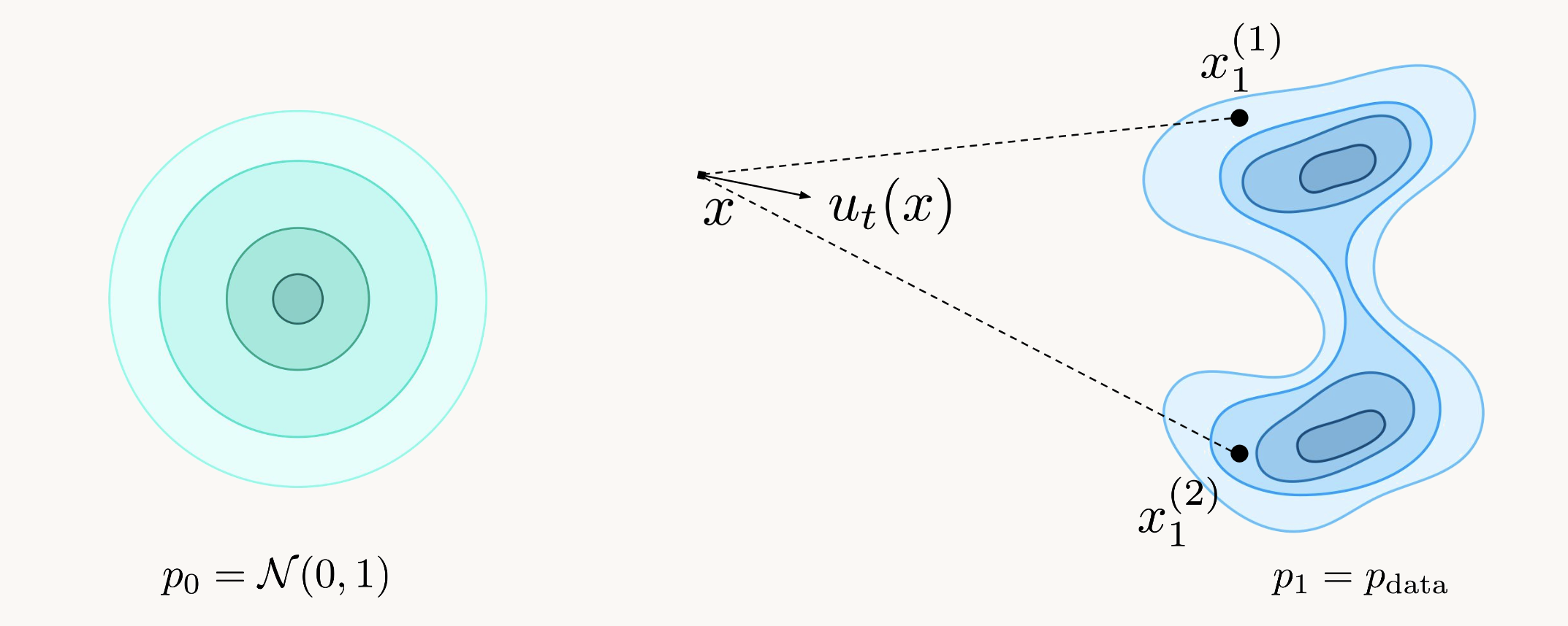
The marginal field $u_t(x)$ can be shown to generate $p_t$ (by respecting the continuity equation above). This means that by following this flow we can transport points from $x_0$ to $x_1$ and cover the whole space (iirc the mapping is bijective if $u_t$ is Lipschitz continuous). It is a weighted average of all conditional fields:

The weight $p(x_1 \mid x_t)$ is the posterior over data points given the current position. It can be interpreted as "given where you are, where could you be heading?"

The problem is that $p_t(x)$ is impossible to compute in practice (i.e. intractable): it is itself an integral over the entire dataset, so there is no way to evaluate $u_t(x)$ from a single sample pair $(x_0, x_1)$. The diagram below shows what this looks like geometrically. An intermediate point $x$ could be on a trajectory heading toward any number of data points $x_1^{(1)}, x_1^{(2)}, \ldots$, each is a plausible direction at any given time.

From any point $x$, many data targets $x_1$ are plausible. The marginal field averages over all of them, weighted by $p_t(x)$, which itself requires integrating over the whole dataset. Intractable.

Conditional flow matching (CFM)

Bear with me for a sec, and let's try to simplify the problem to make it tractable. Let's try fixing a data point $x_1 \sim p_{\text{data}}$ and define a conditional probability path $p_t(\cdot \mid x_1)$ and its conditional vector field $u_t(\cdot \mid x_1)$. These are much easier to specify explicitly. Don't ask why we are doing this, just follow along, it will all become clear. The marginal path is recovered as

By fixing a single $x_1$, the conditional path $p_t(\cdot \mid x_1)$ and its vector field $u_t(\cdot \mid x_1)$ are both easy to specify analytically. The diagram below shows the resulting tractable picture.

Fix one target $x_1$: the path goes straight from noise to that point, and the field $u_t$ is just the direction $x_1 - x_0$. No integration needed.

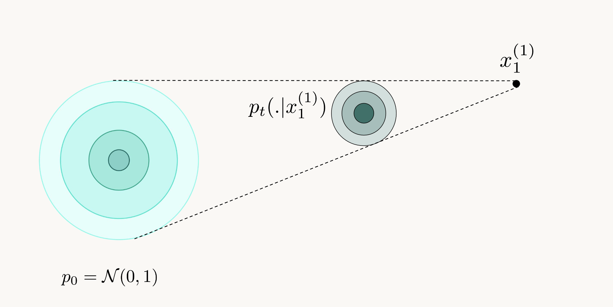
We then train with the conditional flow matching (CFM) loss, which regresses $v_\theta$ to the conditional field on individual samples:

where $x_t \sim p_t(\cdot \mid x_1)$. Now is a good time to answer your burning question: why are we doing this? Feels like we are solving a different problem than the one initially intended. Well, surprise! One can show that the conditional and marginal loss have the same gradient (CME 296, Lecture 3):

So, optimizing the much simpler and tractable CFM loss is exactly equivalent to optimizing the intractable marginal loss. This is what makes flow matching applicable. Feels like magic but it works.

Straight-line paths

We still need to choose the conditional path $p_t(\cdot \mid x_1)$. The simplest valid choice is a straight-line interpolation between noise and data (CME 296, Lecture 3):

The conditional vector field is the time derivative of the path:

This is constant in time; the target velocity does not depend on $t$. The network only needs to learn a displacement, not a time-varying field. Since paths are straight lines we can easily integrate them using Euler's method.

The training objective

Substituting the "straight-line" conditional field into the CFM loss gives the final objective:

Each training step: sample $(x_1, s)$ from data; sample $x_0 \sim \mathcal{N}(0,I)$ and $t \sim U[0,1]$; form $x_t = (1-t)x_0 + tx_1$; regress the network output to $x_1 - x_0$. Couldn't be simpler.

def compute_loss(
    self,
    state: torch.Tensor,
    action_chunk: torch.Tensor,
) -> torch.Tensor:
    action_chunk = action_chunk.reshape(state.shape[0], -1)
    t = torch.rand(
        state.shape[0], 1, device=action_chunk.device, dtype=action_chunk.dtype
    )
    action_gaussian = torch.randn_like(action_chunk)
    a_t = action_chunk * t + (1 - t) * action_gaussian
    target_velocity = action_chunk - action_gaussian
    return F.mse_loss(self._flow_network(state, a_t, t), target_velocity)

Inference: Euler integration

We generate action chunks at test time by starting from $x_0 \sim \mathcal{N}(0,I)$ and integrating the learned ODE using Euler's method with $N$ steps.

After $N$ steps, $x_1 \approx \phi_1(x_0)$ is an approximate sample from $p_{\text{data}}(\cdot \mid s)$. $N=10$ was sufficient to solve the problem.

def sample_actions(
    self,
    state: torch.Tensor,
    *,
    num_steps: int = 10,
) -> torch.Tensor:
    batch_size = state.shape[0]
    flat_chunk_dim = self.chunk_size * self.action_dim
    dt = 1.0 / num_steps
    a_t = torch.randn(
        batch_size, flat_chunk_dim, device=state.device, dtype=state.dtype
    )
    t = torch.zeros(batch_size, 1, device=state.device, dtype=state.dtype)

    for _ in range(num_steps):
        a_t = a_t + dt * self._flow_network(state, a_t, t)
        t = t + dt
    return a_t.reshape(batch_size, self.chunk_size, self.action_dim)

Both policies use the same training infrastructure, implemented in train.py. Since it was my first time using PyTorch and a while since I had implemented a neural network, I played around with a few extras beyond what the homework required:

• Optimizer: AdamW with $\text{lr} = 3 \times 10^{-4}$ and weight decay $\lambda = 10^{-4}$.
• LR schedule: Cosine annealing (no warm-up), decaying from $\text{lr}$ to 0 over the full run.
• Batch size: 128 state-chunk pairs, shuffled each epoch.
• Epochs: 1200. With the Push-T dataset this amounts to roughly 200–220k gradient steps.
• Chunk size: 12 actions per query.
• Noise augmentation: scheduled noise added to training states as a poor man's data augmentation.
• Dropout: 0.1 on the MLP backbone.
• Normalization: states and actions are feature-wise z-scored using dataset statistics; actions are denormalized at evaluation before being clipped to the environment's action bounds.
• Evaluation: 100 fixed-seed episodes in the Push-T gym every 10k steps; mean of per-episode max reward is logged.
• Compilation: torch.compile on the MLP backbone for ~1.4× throughput on MPS.

for epoch in range(config.num_epochs):
    for batch in loader:
        states, actions, noise_scale = batch
        states = states.to(device)
        actions = actions.to(device)
        noise_scale = noise_scale.to(device)
        ...

        loss = model.compute_loss(states, actions)

        optimizer.zero_grad()
        loss.backward()
        optimizer.step()
        if scheduler is not None:
            scheduler.step()

        if step % config.log_interval == 0:
            logger.log({"train/loss": loss.item()}, step=step)
        step += 1

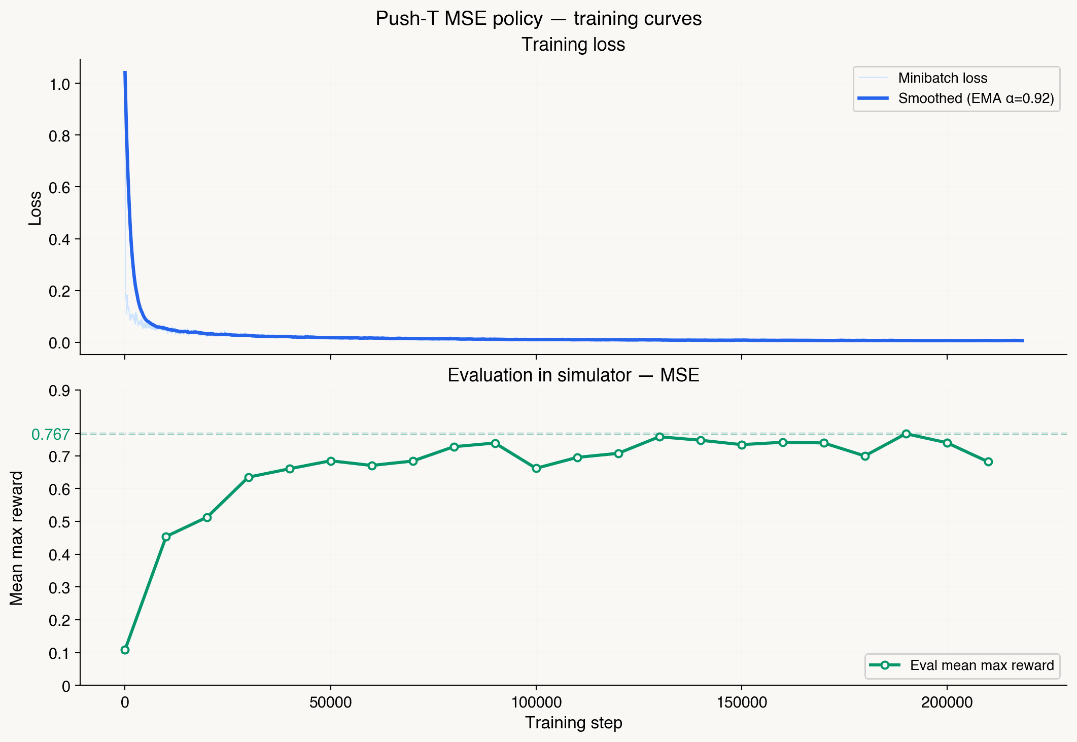
MSE policy peak 0.767

Network. MLP $s_t \mapsto \hat{\mathbf{a}}_t$ with hidden widths $[128, 256, 256, 512]$ (four hidden layers, ReLU, dropout 0.1). Input dim 5 (state), output dim 24 (chunk of 12 × action dim 2). About 240k parameters.

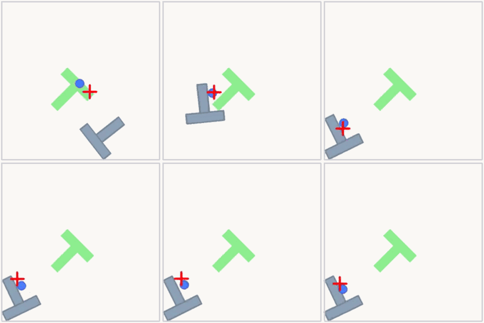
Loss drops sharply in the first few thousand steps then decays slowly toward zero. Reward climbs to ~0.65 within 30k steps and starts oscillating with a peak at 0.767. This does not feel like an optimization problem and more like a fundamental limit.

Increasing network size also had no effect on the problem.

MSE policy, seed 42. Training loss descends from ~1.0 to near zero. Eval mean max reward peaks at 0.767 (dashed line) at step 190k.

MSE policy rollout. Mode averaging produces a mean trajectory that sometimes fits none of the expert modes cleanly.

Why MSE has a ceiling

Minimizing squared error is equivalent to maximum likelihood under a Gaussian model $\pi_\theta(s) = \mathcal{N}(\mu_\theta(s), \sigma^2 I)$. The optimal solution is the conditional mean:

This becomes an issue when the agent has to face a clear decision. Should I approach the object from the left or the right? These are often called homotopy classes (sharp decision boundaries in solution space) and a policy that averages a bunch of trajectories with different homotopies is destined to encounter issues. In other words, the problem is multimodal, and a single modal approach is limited.

What's needed is a policy that can represent the whole distribution over actions, not just its mean. That's what the flow matching policy does.

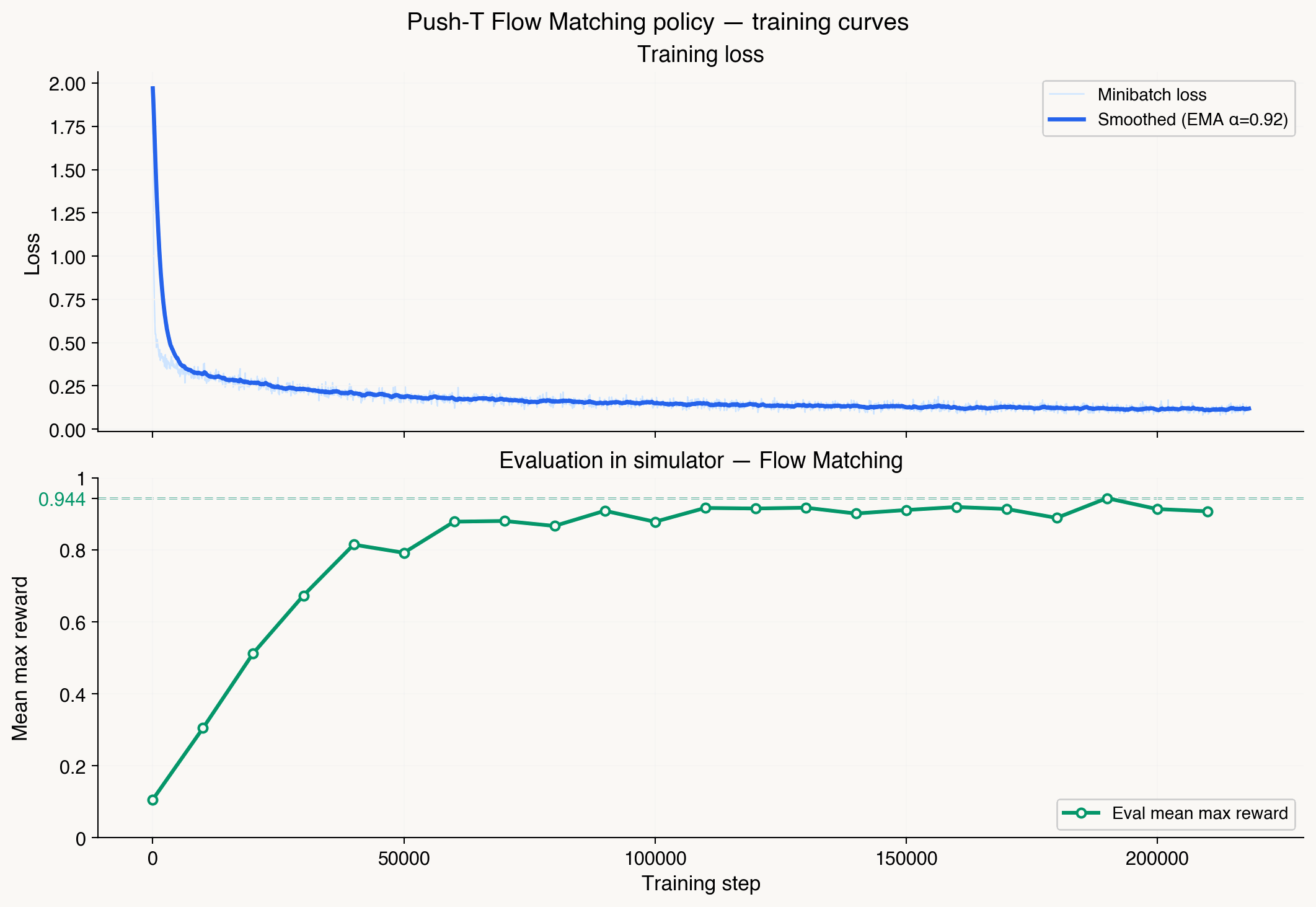
Flow matching policy peak 0.944

Network. MLP $(s, x_t, t) \mapsto v_\theta$ with hidden widths $[128, 256, 512, 512, 512]$ (five hidden layers, ReLU, dropout 0.1). Input dim 30 (state 5 + noisy chunk 24 + time 1), output dim 24. About 700k parameters, roughly 3× the MSE backbone, since the flow head also has to learn the velocity field over $(x_t, t)$.

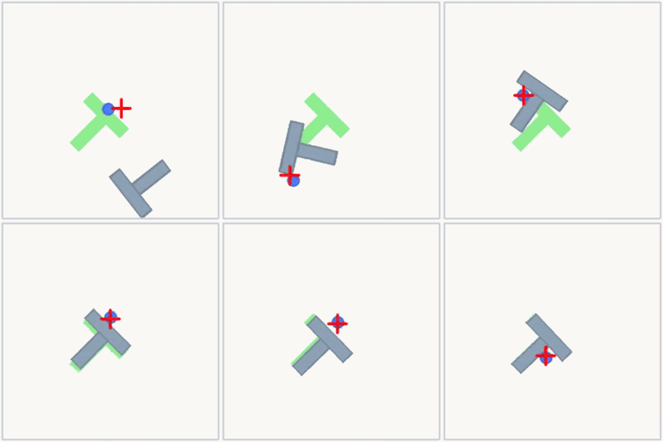
Same optimizer, same number of epochs. Peak eval reward: 0.944, a +0.177 absolute improvement. The difference is entirely structural: the generative policy commits to one mode per episode rather than averaging over all of them.

Flow matching policy, seed 42. Training loss falls from ~2.0 to ~0.15 (different scale from MSE; the flow target is $x_1 - x_0$, not the action directly). Eval reward peaks at 0.944 (dashed line) and stays above 0.90 after step 60k.

Flow matching rollout. The agent picks a side and commits. Motion is smooth and decisive, exactly what mode-specific sampling enables.

This was a great little project to get your feet wet in RL. I really enjoyed applying flow matching after having studied it not too long ago. I was surprised how easy the setup was in PyTorch. After 10 years of C++, I forgot all about the ease of interpreted languages with mature libraries. Overall, I was very impressed with the performance of BC and finally understand why it has been such a widely adopted technique in AV.

• CS 285 Deep RL, UC Berkeley. Lectures 2–3: Behavioral Cloning. Spring 2026. rail.eecs.berkeley.edu/deeprlcourse. Covers behavioral cloning, distribution shift, DAgger, and generative action policies.
• Stanford CME 296. Lecture 3: Flow Matching. Spring 2026. cme296.stanford.edu. Motivation, probability paths, conditional flow matching, parallel with diffusion and score matching.

If you made it this far you deserve a break. Try running the secret shell ./he_yeah.sh in the terminal of the homepage.