Q-Learning - DQN

We left off the previous note with the off-policy actor-critic below: a critic $Q_\varphi(s, a)$ fit by regression, and an actor trained, through the reparameterized policy gradient, to pick actions that make $Q_\varphi$ large.

As I flagged there, this was a pedagogical derivation, meant to show the bridge from policy gradient to a Q-critic, not something you would implement as-is. This page takes the discrete-action case and turns it into something that actually runs.

Look again at that algorithm, and notice that the actor is really just an optimizer. Its whole job is to produce, at each state, the action that makes $Q_\varphi$ as large as possible, and the reparameterized policy gradient is what trains it to do exactly that. So the question is whether we can skip the actor and take that max directly.

It would be great if we could, and whether we can comes down to the action space.

• Discrete actions. We can take the max naively. One forward pass reads off $Q_\varphi(s_i', \cdot)$ for every action, and we keep the best: $$\mathbb{E}_{a' \sim \pi_\theta}\big[Q_\varphi(s_i', a')\big] \;\to\; \max_{a'} Q_\varphi(s_i', a').$$ There is nothing left for the actor to do. We delete it and read the policy straight off $Q$. This is the case we build out here.
• Continuous actions. You cannot enumerate the actions, so that max becomes its own optimization problem at every step. The usual fix is to keep an explicit actor whose job is to approximate $\arg\max_{a'} Q_\varphi$ (that is DDPG, TD3, and SAC), which I will cover in a follow-up page. Everything here still applies there: it is the same Bellman target, just with the max done by a network instead of by enumeration.

The discrete branch is Q-learning: an off-policy method with a single network, no policy gradient, and the actor replaced by an $\arg\max$. The rest of this page makes it precise, shows why the max is justified, adds the tricks that make it actually train, and ends with some fun results on Ms. Pac-Man, following HW3 of the course.

With the risk of repeating myself, let's make that collapse precise and write it as a standalone algorithm, because it is the source of everything here. If we look again at the bootstrap target:

Which policy makes that expectation as large as possible? The greedy one: at every state pick the action with the highest $Q$. If we simply define our policy to be that greedy policy,

then the expectation collapses to a max, $\mathbb{E}_{a' \sim \pi}[Q_\varphi(s', a')] = \max_{a'} Q_\varphi(s', a')$, and the target becomes

The actor is gone. We no longer train a $\pi_\theta$, and there is no policy gradient or second network. The policy is just the argmax of $Q$, which leaves a single loop:

We could honestly stop here, this is already a working idea. But it is worth understanding why taking the max gives a better policy. That comes from the classical tabular theory, so let me go through it.

The max is doing policy improvement. To see why, go back to the tabular case where everything is exact, with small discrete state and action sets, known dynamics, and one value stored per state. Sutton & Barto chapter 4 has the full proofs, here I will just give the idea.

Policy iteration repeats two steps:

• Policy evaluation: compute $Q^\pi$ (or $V^\pi$) for the current policy.
• Policy improvement: set $\pi' (s) = \arg\max_a Q^\pi(s, a)$, the greedy policy for the values you just computed.

The policy improvement theorem says this greedy policy is at least as good as $\pi$ at every state, so each round can only make the policy better, and in the tabular case it ends at the optimal policy. Evaluation itself is a simple update: plug the current estimate back in on the right and sweep:

Value iteration does both steps at once, so you never store a policy at all:

The $\max$ here is the policy improvement step, since the value of the greedy policy is just the max over actions. This is where Q-learning comes from. The Q-learning target from the last section is the same update, with $\max_{a'} Q(s', a')$ in place of $V(s')$.

Tabular methods only work when you can store one number per state, which is hopeless for real problems. An image observation has something like $|\mathcal{S}| = (255^3)^{200 \times 200}$ states, far too many to enumerate, let alone store. This is the curse of dimensionality. The fix is to replace the table with a function approximator $V_\varphi : \mathcal{S} \to \mathbb{R}$ and fit it by regression onto the value-iteration target:

There is a catch that rules this out for model-free RL. Computing $y_i$ needs the $\max_a$ over actions and the $\mathbb{E}$ over $s'$, and both require knowing the outcome of every action from $s_i$. With a state-value function you only stored the one action you actually took, so you cannot evaluate the alternatives without a model $p(s' \mid s, a)$ to simulate them. Sadly we generally do not have one, but that is also what makes RL powerful.

The fix is the same one we used to cross the bridge: learn $Q$ instead of $V$. With a Q-function we approximate the next-state value by the network's own max,

and now the max is over the network's outputs at $s_i'$. No model and no simulating actions. One forward pass gives $Q_\varphi(s_i', \cdot)$ for all actions and we take the max. The target is

This is clearly off-policy as the $(s, a, s')$ data does not need to match the current policy. The main question is: what is it actually optimizing? Define the Bellman error

If $\mathcal{E} = 0$ then $Q_\varphi(s, a) = r(s, a) + \gamma \max_{a'} Q_\varphi(s', a')$ everywhere, which is the Bellman optimality equation. Its unique solution is the optimal Q-function $Q^\star$, and the greedy policy on $Q^\star$ is the optimal policy $\pi^\star$. So in the tabular case fitted Q-iteration is exactly solving for the optimum. Once $Q_\varphi$ is a neural net, though, most of these guarantees are lost, which is the first sign of trouble we will come back to.

Fitted Q-iteration gathers a big batch then fits. The downside is you collect all that data before doing any learning, so you spend a long time acting on an old policy. Online instead updates after every step, so the policy improves as you go. Each iteration is one transition followed by one gradient step:

Which action do we take in the first step? The final policy is greedy, $\arg\max_a Q_\varphi(s, a)$, but using the greedy policy to collect data is a bad idea. It is deterministic, so it will keep exploiting whatever looks best early and never try the actions it is currently underrating, which means it never finds out they were good. We need to explore. Two standard choices:

• Epsilon-greedy: take the greedy action with probability $1 - \epsilon$, otherwise a uniformly random one. $$\pi(a \mid s) = \begin{cases} 1 - \epsilon & a = \arg\max_a Q_\varphi(s, a) \\ \epsilon / (|\mathcal{A}| - 1) & \text{otherwise} \end{cases}$$
• Boltzmann: sample softly in proportion to value, $\pi(a \mid s) \propto \exp(Q_\varphi(s, a))$. Near-best actions get tried often, clearly bad ones rarely.

In code this is the whole of get_action: take the argmax of $Q_\varphi$, then with probability $\epsilon$ swap in a uniformly random action instead.

with torch.no_grad():
    q_values = self.critic.forward(observation)
max_action = torch.argmax(q_values, dim=1).item()

if np.random.rand() < 1 - epsilon:
    return max_action
else:
    rand_actions = np.arange(self.num_actions)
    rand_actions = rand_actions[rand_actions != max_action]
    return np.random.choice(rand_actions)

Because Q-learning is off-policy, we can explore like this and still be learning about the greedy policy. The behavior policy that collects data and the policy we are improving do not have to match. Exploration gets a whole lecture of its own later, this is enough to get going.

Combine the pieces: collect with an exploratory policy, store transitions in a replay buffer, and run Q-learning updates on batches sampled from it.

This is, in spirit, DQN. But if you code exactly this up, it most likely won't work. There are 3 main issues with this algorithm, and I will now address them in detail in the next sections.

Write the online update as a gradient step and look at what is inside it:

The bracket is the target $y_i$, and it contains $Q_\varphi$ too. We hold it constant and do not differentiate through it, so this is a semi-gradient (as we saw before), not the gradient of any fixed loss. And because the target is built from the same network, it moves the instant we step $\varphi$. There is no fixed target to converge to.

The fix is a target network: a second copy $Q_{\bar\varphi}$ with frozen parameters $\bar\varphi$, used to build the target,

refreshed $\bar\varphi \leftarrow \varphi$ only every $N$ steps (10,000 is typical). Between refreshes the labels hold still, so each window is a well-defined regression onto fixed targets. The target still moves, just slowly, which is enough to keep the whole thing from diverging.

In code the target network is just a second copy of the critic, refreshed on a fixed period:

def update_target_critic(self):
    self.target_critic.load_state_dict(self.critic.state_dict())

# inside DQNAgent.update(...), once per gradient step:
critic_stats = self.update_critic(obs, action, reward, next_obs, done)
if step % self.target_update_period == 0:
    self.update_target_critic()

A one-step target moves reward back just one state per target refresh. Picture a long corridor with the only reward at the far end and $Q_{\bar\varphi}$ starting at zero: the first update raises $Q$ at the last state, the next refresh reaches the one before it, and so on. A reward $n$ steps away needs about $n$ refreshes to reach the start, which is slow, and slower still since the target is only refreshed every $N$ steps.

The fix is to carry more real reward in each target before bootstrapping. Sum the next $n$ rewards, then bootstrap from there:

Now reward propagates $n$ steps per update, and the early target leans more on real rewards than on the network's initial estimate, so learning is faster and less biased at the start. It is the same bias / variance dial as the GAE story on the actor-critic page, applied to a $Q$-target. People do use the GAE form here too: instead of committing to one $n$, exponentially weight all the $n$-step returns into a $\lambda$-return, as in Q($\lambda$) or Retrace. A fixed small $n$ is simpler and the more common choice in deep Q-learning.

The final issue is that Q-learning systematically overestimates. If you plot the predicted value against the return the policy actually earns and the prediction is generally higher, sometimes by a lot.

The reason is the $\max$ in the target. For any set of noisy estimates, Jensen's inequality gives

The $Q_{\bar\varphi}(s', \cdot)$ are noisy, and the $\max$ picks out whichever $Q$ has the higher noise, so each target is generally higher than it should be. That inflated target is then what the next update regresses toward, creating a bad feedback loop.

We can see this more clearly by writing the $\arg\max$ explicitly as a function of $Q$:

The same network picks the action and scores it, so it grades its own choice with the very noise that made it pick, and the error does not average out.

Double Q-learning breaks that correlation, one network picks and a different one scores. We already have two from the target network above, so let the current $Q_\varphi$ pick and the target $Q_{\bar\varphi}$ score:

In code this is simply implemented as:

with torch.no_grad():
    next_target_qa_values = self.target_critic.forward(next_obs)

    if self.use_double_q:
        next_critic_qa_values = self.critic.forward(next_obs)
        next_action = torch.argmax(next_critic_qa_values, dim=1)
    else:
        next_action = torch.argmax(next_target_qa_values, dim=1)

    next_q_values = next_target_qa_values[batch_idx, next_action.long()]
    target_values = reward + self.discount * (1 - done.float()) * next_q_values

Stacking the three fixes onto the naive version gives DQN in full. Each line ties back to one of the issues above.

Before getting to the results, let's take a little step back and summarize the different flavors of Q-learning we have discussed so far. All those names confused me when I first went through the lectures, so I wanted to make them extra clear. To do that, let's highlight the 3 main processes of the algorithm:

• Process 1, data collection. Act in the world, push $(s, a, s')$ into the buffer, evict old data when full.
• Process 2, target update. Copy the parameters into the target network, $\bar\varphi \leftarrow \varphi$.
• Process 3, regression. Sample a batch and take a gradient step on $Q_\varphi$ toward the targets.

Now each Q flavor is as follows:

• Online Q-learning. Buffer of size one. All processes run in lockstep, so the target moves every step. Least stable but most reactive.
• DQN. Processes 1 and 3 run together, process 2 is slow (target copied every $N$ steps).
• Fitted Q-iteration. Fully nested: collect a big dataset, then for each frozen target run many regression steps. The most stable, the least online.

With one knob per loop they are the same pseudocode:

DQN is just $N = 1,\ K = 1$ (but with a sizeable replay buffer and batch). Fitted Q-iteration is big $N$ with a $K$-step inner regression. Online Q-learning uses the same $N = 1,\ K = 1$ as DQN, the only difference being that the replay buffer holds a single transition instead of a large pool.

Here are a few implementation tips given by the course and used throughout the code.

Start simple. Test your code on simple and fast problems first, add features incrementally. RL is not easy to debug.

Large replay buffers. Consider large replay buffers. This will come at the cost of more compute but should be more stable.

Huber loss. The TD error can be large early on. A gentler cost for tail events is the Huber loss on the TD error $e = y - Q_\varphi(s, a)$,

quadratic near zero and linear in the tails, so a handful of huge errors pull the gradient less hard. The code currently uses a plain MSE (nn.MSELoss), so this is a swap you could make, not what is running.

Gradient clipping. Another guard against large TD errors. After backward() the critic's gradient norm is clipped (to 10 for Atari) before the optimizer step, which keeps the update direction but caps its magnitude:

loss = self.critic_loss(q_values, target_values)

self.critic_optimizer.zero_grad()
loss.backward()
grad_norm = torch.nn.utils.clip_grad.clip_grad_norm_(
    self.critic.parameters(), self.clip_grad_norm or float("inf")
)
self.critic_optimizer.step()

Anneal exploration and the learning rate. Start with high exploration and decay $\epsilon$; schedule the learning rate down too. Both are annealed on the same kind of piecewise schedule, held flat through the 20k-step warmup, then ramping linearly to their floor at the halfway point of training: $\epsilon$ from 1 down to 0.01, and the learning rate from full to half.

def make_lr_schedule(optimizer: torch.optim.Optimizer) -> torch.optim.lr_scheduler._LRScheduler:
    return torch.optim.lr_scheduler.LambdaLR(
        optimizer,
        PiecewiseSchedule(
            [
                (0, 1),
                (20000, 1),
                (total_steps / 2, 5e-1),
            ],
            outside_value=5e-1,
        ).value,
    )

exploration_schedule = PiecewiseSchedule(
    [
        (0, 1.0),
        (20000, 1),
        (total_steps / 2, 0.01),
    ],
    outside_value=0.01,
)

Multiple seeds and patience. Run multiple seeds and be patient, it can take a while to converge. Q-learning can be inconsistent between runs.

The result below is a single DQN agent trained on Ms. Pac-Man (MsPacmanNoFrameskip-v4) straight from pixels. After the standard DeepMind Atari wrappers the observation is four stacked $84 \times 84$ grayscale frames, and the action set is the discrete joystick directions, so the policy stays implicit as $\arg\max_a Q_\varphi(s, a)$ with no actor anywhere.

The hyperparameters are the ones from the HW3 Atari config:

• Q-network: the original DQN convolutional stack, three conv layers (32, then 64, then 64 channels) into a 512-unit dense layer and a linear head to the action values $Q_\varphi(s, \cdot)$.
• Optimizer: Adam, $\text{lr} = 10^{-4}$, with the linear decay to $0.5\times$ from the schedule above.
• Discount: $\gamma = 0.99$.
• Batch size: 32, sampled from the replay buffer each step.
• Target network: hard copy every 2000 steps.
• Double Q: on. Gradient clipping: norm 10.
• Exploration: $\epsilon$ annealed from 1.0 to 0.01 on the schedule above.
• Warmup: 20,000 random steps before learning starts.
• Total steps: 1,000,000, single seed.

The run is one command on the Ms. Pac-Man config:

uv run src/scripts/run_dqn.py -cfg experiments/dqn/mspacman.yaml

With all the pieces in place, here is the agent early in training and after about 1M steps:

Early
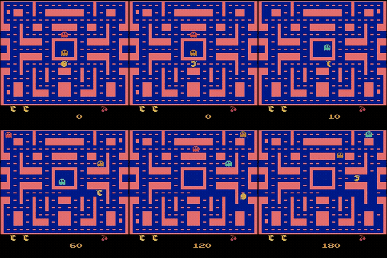
~50k steps

Trained
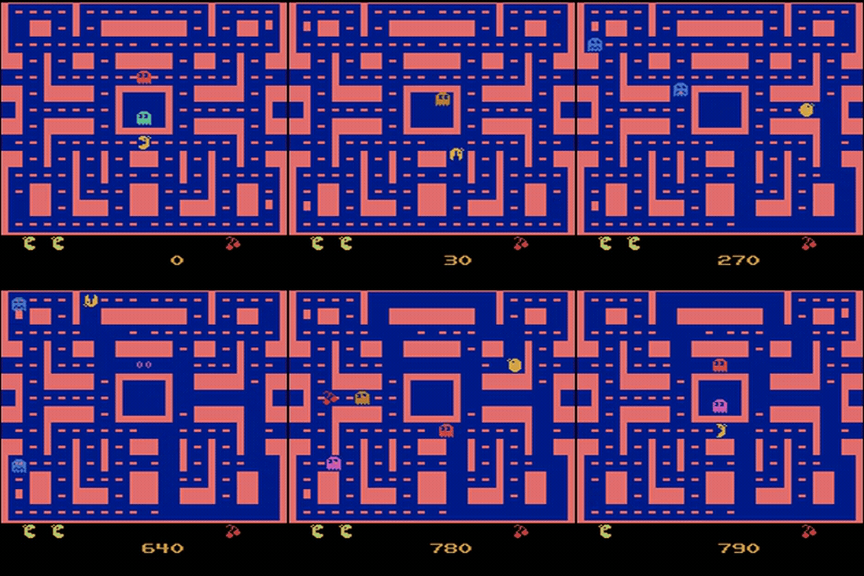
~1M steps

The lecture asks a good question about these agents. Does the predicted $Q$ actually mean anything? If it does, the mean predicted $Q$ and the mean eval return should be directly correlated and follow the same trend over training. They are not 1:1 in magnitude though: the eval return is the full episode total, while $Q$ is a discounted estimate of the return from a state anywhere along the trajectory, including tail states near the end where little reward is left, and then averaged over many such states. So same trend but different scale.

Ms. Pac-Man DQN, 1M steps, single seed. Top: eval return, climbing from ~60 to a smoothed ~1800 (peak 2465). Bottom: mean predicted $Q$, climbing from 0 to ~158. They move together which indicates that the value estimate is tracking real return rather than hallucinating.

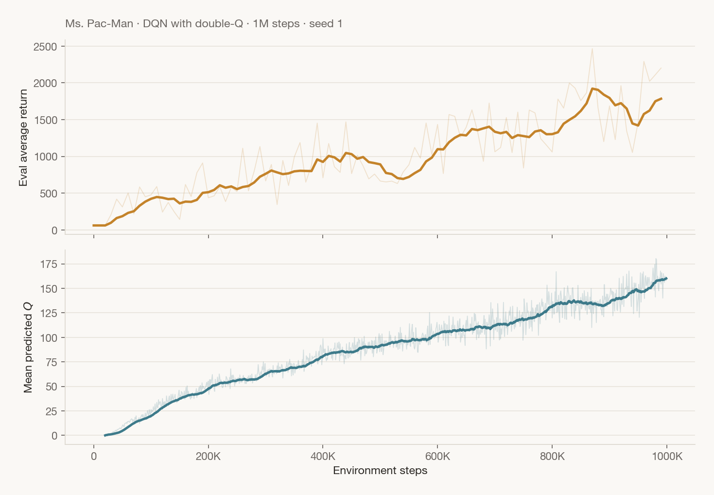
It is one seed and it is still climbing at 1M steps indicating that the algorithm is working properly.

The full DQN agent, the Atari wrappers, and the training script can be found here.

We went from on-policy to off-policy with one move: let the value function take the action as an input ($Q$ instead of $V$). That is what lets the bootstrap use the current policy on old data. For discrete systems we can just use the greedy max as a policy and throw the actor in the trash. This is the essence of pure value-based DQN.

The naive version does not train, but the fixes are small. A target network freezes the regression target so we are not chasing ourselves. $n$-step returns move reward back faster, and double Q-learning splits the max from the argmax and removes the overestimation bias. If we stack those we get a working DQN, the Ms. Pac-Man agent above.

We also discussed the online / fitted / DQN spectrum and showed it is all one loop at different speeds.

This is it for discrete actions. We will consider next how to handle continuous actions, where the argmax operator is not obvious and becomes its own optimization. Everything we learned here will still apply though!

• CS 285 Deep RL, UC Berkeley. Lecture 7: Value-Based RL (PDF) and Lecture 8: Q-Learning in Practice (PDF, target networks through double Q-learning). rail.eecs.berkeley.edu/deeprlcourse.
• Sutton & Barto. Reinforcement Learning: An Introduction, 2nd ed. PDF. Chapter 4 (dynamic programming, policy and value iteration, the policy improvement theorem) and §6.5 (Q-learning).
• My implementation: CS_285_Deep_RL / hw3 (DQN and SAC).

If you read all the way through, you have earned a classic. Run ./run_me.sh in the terminal on the homepage.