Continuous Q-Learning - DDPG, TD3, SAC

DQN uses the max over actions in two places: to act, and to build the target,

As we have seen in the previous page, with a discrete action set the policy is trivial: we forward pass the network to get every $Q(s, a)$ at once and take the largest. With a continuous action $a \in \mathbb{R}^d$ each max becomes a nonlinear, and in general non-convex, optimization problem over the action ($Q_\varphi$ is a neural network in $a$). This optimization problem can be costly which becomes an issue especially when building the target as this needs to be solved at every transition of every batch, on every gradient step. We therefore need a faster method.

The simplest fix is to approximate the max with samples,

This is the naive approach and parallelizes well into one batched forward pass. This however is not very accurate for large number of actions as the discretization error can be large.

There are some more accurate iterative versions:

• The cross-entropy method (CEM). Sample some actions from a Gaussian, keep the best few, and move the Gaussian toward them. Repeat a few times so the samples close in on the high-$Q$ actions.
• CMA-ES. The same loop, but it also adjusts the shape of the Gaussian, not just its center. A bit more accurate, a bit more compute.

These work OK up to roughly 40 action dimensions ($\dim \mathcal{A} \approx 40$) but tend to have accuracy issues afterward. This search also has to be redone from scratch every state, meaning every transition in the batch. This can become quite costly.

Accuracy is not a massive issue when building the target as it is a noisy estimate anyway, but we would like the action selection to be as good as possible. Thankfully we can approximate the argmax with its own neural network and this is what this page builds on as we will see below.

The max is just the $Q$-value at the argmax,

so the idea is to train a second network to output the argmax,

A network that maps a state to the best action is a deterministic actor, so we are back to actor-critic. And training it is an optimization we can do with gradients. $\mu_\theta$ should maximize the critic,

which by the chain rule moves $\theta$ in whatever direction the critic says raises $Q$.

The critic target then uses the actor $\mu_{\bar\theta}$ in place of the argmax, and just like DQN froze the critic into $Q_{\bar\varphi}$, we also freeze the actor into $\mu_{\bar\theta}$. Both frozen copies are there for the same reason: to hold the regression target still. If the target used the live $\mu_\theta$, the target action would move on every actor update and the critic would chase a shifting target.

Sadly the overestimation that double Q-learning partially fixed is back. The actor's job is to maximize the critic, so it seeks out exactly the overly-optimistic actions, and the target picks them up. We will see how to address that in TD3 below.

Put together this is DDPG (deep deterministic policy gradient):

Two little things to note:

• The actor is fully deterministic so it explores nothing by itself. Instead the noise used when collecting data fills the role $\epsilon$-greedy had in DQN.
• The target networks are updated softly using Polyak averaging (the last line above), $\bar\varphi \leftarrow \tau\varphi + (1-\tau)\bar\varphi$. Each step nudges the target a little toward the online network rather than making one large jump every $N$ steps, so the target moves smoothly instead of in sawtooth steps.

Remember from the Q-learning notes that by Jensen's inequality $\mathbb{E}[\max] \ge \max \mathbb{E}$, so the max over a noisy $Q$ overestimates. We previously fixed this by decorrelating action selection from evaluation, using a different network for each (live vs target network).

With the learned argmax the networks for selection and evaluation are decorrelated in terms of noise, but the overestimation problem might be worse than before: the actor is explicitly trained to maximize the critic, so it seeks out actions where the critic is too optimistic, and the bootstrap then propagates those inflated values everywhere.

TD3 (twin delayed DDPG) addresses this issue with clipped double-Q: train two critics side by side and let the target take the minimum,

Taking the min of two noisy estimates is biased low rather than high, and here biasing low is the safe side: the actor cannot exploit an error unless both critics happen to share it.

TD3 adds two more fixes on top of DDPG:

• Clipped noise on the target action, $a' = \mu_{\bar\theta}(s') + \epsilon$ with $\epsilon$ clipped to a small range. The critic is a neural net, so it can have narrow bumps where it wrongly rates one action too high. The actor always picks the highest-rated action, so a single $a'$ lands right on that bump and the target copies the wrong value. The noise spreads $a'$ over a few nearby actions instead of one, which averages the bump out and keeps close actions at close values.
• Delayed actor updates: step the actor (and the target networks) once every two critic steps instead of every step. The actor's loss is to maximize $Q_\varphi(s, \mu_\theta(s))$, so each actor step moves the policy straight toward wherever the critic is high, errors included. Letting the critic settle for a couple of steps first means the actor chases a more accurate value, so its mistakes do not compound.

In the HW3 implementation the critics are an ensemble, and we either average them or take the min:

if self.target_critic_backup_type == "mean":
    next_qs = next_qs.mean(dim=0)
elif self.target_critic_backup_type == "min":
    next_qs = next_qs.min(dim=0).values

DDPG made the actor deterministic to imitate the argmax. SAC (soft actor-critic), on the other hand, keeps the actor stochastic. The actor is a Gaussian $\pi_\theta(a \mid s) = \mathcal{N}\big(\mu_\theta(s),\, \sigma_\theta(s)\big)$, the same form as the off-policy actor-critic notes.

SAC adds an entropy bonus to encourage the actor to be more random. That bonus is maximized alongside the return, scaled by a temperature $\alpha$:

The entropy term always pushes the same way, toward a more spread-out policy, so it is a constant nudge to explore. The return pushes back by rewarding the best action. When the $Q$ values are close, staying random costs almost no return, so entropy wins and the policy stays broad. When one action is clearly best, its return gain outweighs the lost entropy, so the policy focuses on it. This is a nice mechanism where the actor ends up random exactly where it is unsure which action is best.

The temperature $\alpha$ is the Pareto term determining how balanced the interaction is between entropy maximization and deterministic action maxing. A larger $\alpha$ means there needs to be a large gap in $Q$ value before the policy collapses to one action, and a smaller $\alpha$ lets it collapse more easily.

The actor

The actor is a squashed Gaussian, sampled with the reparametrization trick:

The $\tanh$ keeps actions in $[-1, 1]$ (the control limits). Writing the sample as a deterministic function of the noise, $a_\theta(s, \epsilon) = \tanh\big(\mu_\theta(s) + \sigma_\theta(s) \odot \epsilon\big)$, is what lets us take the gradient. The actor wants to raise $Q$, that is, maximize $\mathbb{E}_{s \sim \mathcal{D},\, a \sim \pi_\theta}[Q(s,a)]$. The trouble is the distribution we average over depends on $\theta$, so we cannot push $\nabla_\theta$ straight inside. Reparametrizing moves the $\theta$-dependence out of the distribution and into the integrand, where the expectation is now over the fixed noise $\epsilon$:

The last step swaps $\nabla_\theta$ with the expectation, which is now allowed because $\epsilon$'s distribution has no $\theta$ in it. The inner $\nabla_\theta Q$ is the same DDPG chain rule $\nabla_a Q \cdot \nabla_\theta a_\theta$, only on a random action instead of a deterministic one. SAC adds the entropy term to this, and minimizing the negative of the whole objective gives the actor loss, estimated with one sample per state:

where $-\log \pi_\theta(a \mid s)$ at a sampled action is the one-sample entropy estimate.

In code, the actor samples an action and reads its $Q$:

# Sample from the actor
action_distribution: torch.distributions.Distribution = self.actor(obs)

action = action_distribution.rsample()
q_values = self.critic(obs, action)

loss = -q_values.mean()

The entropy bonus is subtracted one level up, in update_actor, and the entropy itself is a single reparametrized sample:

loss, entropy, log_prob = self.actor_loss_reparametrize(obs)

loss -= self.temperature * entropy

return -action_distribution.log_prob(action_distribution.rsample())

The critic

The entropy also goes into the critic target, so the $Q$-function values the randomness of future actions too, not just future reward:

As on the off-policy actor-critic page, the transition is old but $a'$ is sampled fresh from the current policy, which is what makes the whole thing off-policy safe. In code:

# Compute target values
with torch.no_grad():
    next_action_distribution = self.actor(next_obs)
    next_action: torch.Tensor = next_action_distribution.sample()
    next_qs = self.target_critic(next_obs, next_action)

    if self.use_entropy_bonus and self.backup_entropy:
        next_action_entropy = self.entropy(next_action_distribution)
        next_qs += self.temperature * next_action_entropy

then target_values = reward + self.discount * (1 - done) * next_qs and a squared-error fit, same as every critic before it. The full loop:

A fixed $\alpha$ is one more hyperparameter to tune per environment, and the right amount of randomness changes over training (a lot early, little late). The SAC authors' fix is to state what we actually want as a constraint: maximize return, subject to the policy keeping at least some minimum entropy,

with the target entropy usually set to $\mathcal{H}_{\text{tgt}} = -\dim(\mathcal{A})$.

We can solve this with dual ascent after forming the Lagrangian with $\alpha \ge 0$ as the Lagrange multiplier on the entropy constraint. The primal steps are the actor and critic updates above, run at the current $\alpha$. The dual step then updates $\alpha$ by ascending along the constraint slack $\mathcal{H}_{\text{tgt}} - \mathcal{H}(\pi_\theta)$:

When entropy sits below the floor, $\mathcal{H}(\pi_\theta) < \mathcal{H}_{\text{tgt}}$, the slack is positive and $\alpha$ climbs to buy back exploration; above the floor $\alpha$ falls. In code $\alpha$ is kept positive by optimizing $\log \alpha$, which also removes the projection $[\,\cdot\,]_+$. Minimizing

is just a way to get that dual step out of the optimizer. Its gradient with respect to $\log \alpha$ is $\mathcal{H}(\pi_\theta) - \mathcal{H}_{\text{tgt}}$, so descending it moves $\log \alpha$ by the same slack $\mathcal{H}_{\text{tgt}} - \mathcal{H}(\pi_\theta)$ that drives the ascent above: same direction, same fixed point $\mathcal{H}(\pi_\theta) = \mathcal{H}_{\text{tgt}}$ (the note below has the subtlety). This is the form the code uses:

alpha = torch.exp(self.log_alpha)
alpha_loss = -(self.log_alpha * (log_prob + self.target_entropy).detach()).mean()

self.alpha_optimizer.zero_grad()
alpha_loss.backward()
self.alpha_optimizer.step()

Putting the temperature update alongside the actor and critic steps gives the full recap:

The lecture closes with a theory result I will just summarize. In the tabular case the Bellman update is a contraction: every iteration shrinks the distance to $Q^\star$ by $\gamma$, so value iteration provably converges. With a neural network each update is followed by a projection onto the functions the network can represent, and although both steps are contractions, they are in different norms, so their composition is not. So none of the fitted methods here (DQN, DDPG, TD3, SAC, and the critic of any actor-critic) comes with a convergence guarantee: values can oscillate or diverge, and the tricks we keep adding (target networks, big replay buffers, double-Q) do not restore the guarantee, they just make failure rarer in practice.

The result below is SAC trained on HalfCheetah-v4 (MuJoCo), the same environment as the policy gradient experiments: a 17-dimensional state and 6 continuous joint torques, rewarded for forward speed. The hyperparameters are the ones from the HW3 config:

• Actor: tanh-squashed Gaussian with state-dependent std, 3-layer MLP, 256 units per layer.
• Critic: $Q_\varphi(s, a)$ MLP of the same size, taking the state and action as input.
• Optimizer: Adam, $\text{lr} = 3 \times 10^{-4}$ for both networks. Batch size: 256.
• Discount: $\gamma = 0.99$. Target update: soft, $\tau = 0.005$.
• Entropy: two runs, one at fixed temperature $\alpha = 0.1$ and one with automatic temperature, entropy in both the actor loss and the critic target.
• Total steps: 1,000,000, with 5,000 random warmup steps and learning starting at 10,000. Eval every 5,000 steps, averaged over 10 episodes.

The run is one command on the HalfCheetah config:

uv run src/scripts/run_sac.py -cfg experiments/sac/halfcheetah.yaml

Here is the SAC agent during the random warmup and after 1M steps:

Early
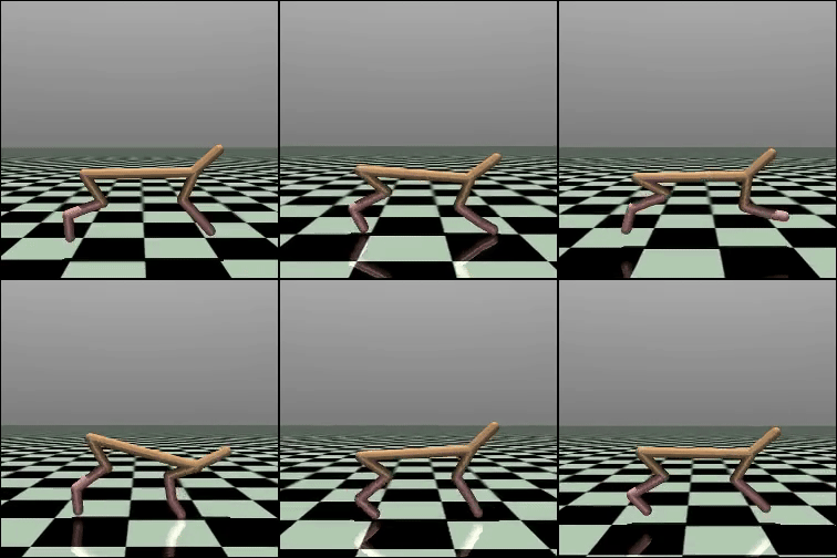
~5k steps

Trained
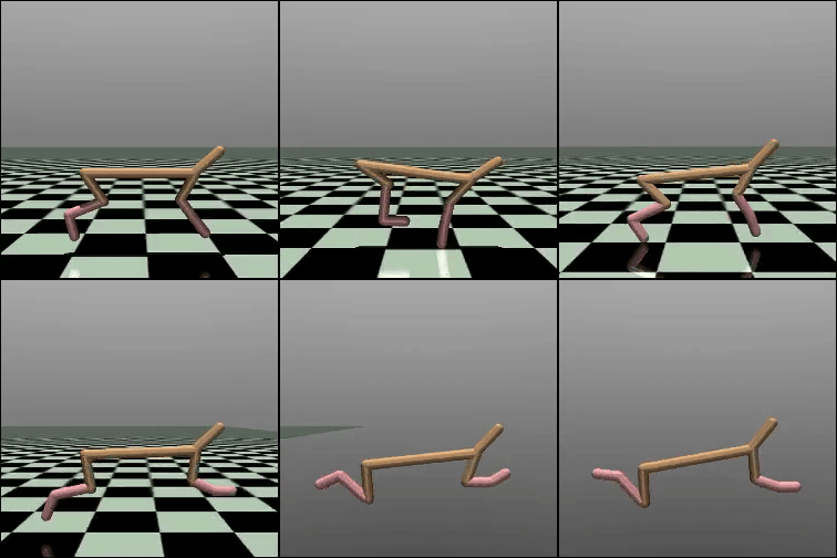
~1M steps

The trained agent moves far better than the plain policy gradient runs from the earlier notes, where the same cheetah topped out around a peak return of 739.

I ran two experiments: plain SAC with a fixed temperature, then SAC with the temperature tuned automatically by dual ascent. Both are below.

Result 1: fixed temperature

Here the temperature stays fixed at $\alpha = 0.1$ for the whole run. I trained the same config twice (both seed 1; the runs still differ a little because the GPU floating-point reductions are not run-to-run deterministic). Both climb steadily to a smoothed eval return just under 10,000, with the best single evals around 10,300. Training looked stable to me: the two runs stay close together the whole way, with no plateau.

HalfCheetah-v4, SAC, 1M steps, two runs of the same config. Top: eval average return, faint line is the raw eval, thick line a trailing average, the dot marks the smoothed peak. Bottom: policy entropy over training.

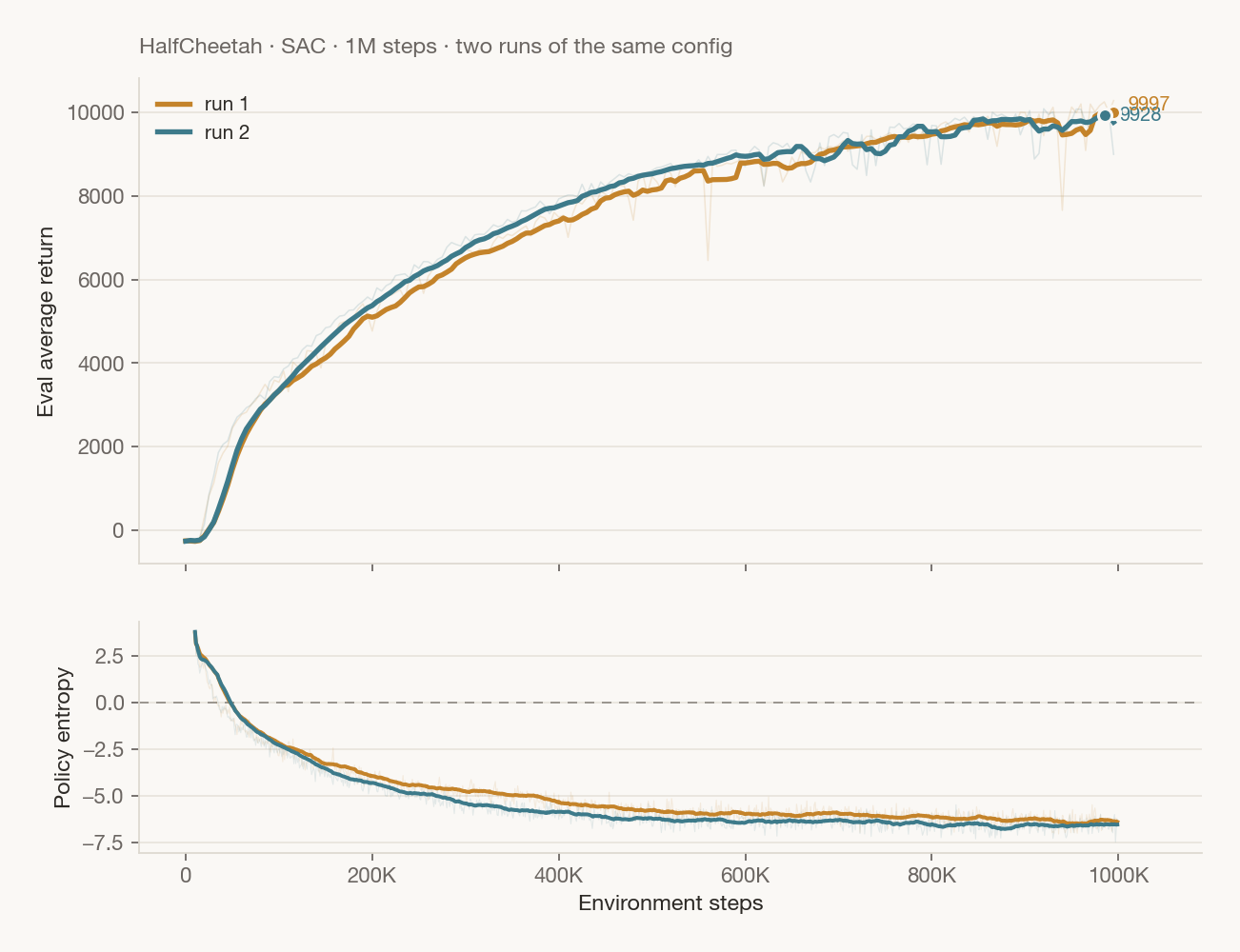
The bottom panel shows the policy entropy. It starts pretty high, around 4.2 nats (roughly $6 \log 2$), an almost uniform policy, and falls as the policy grows more confident, settling around $-6.5$ (this is differential entropy of a continuous density, so it can go negative, see the information theory notes). Where it settles is set by the balance between $\alpha$ and the reward scale: with $\alpha$ fixed, the $Q$-values grow over training, so the entropy bonus matters less and the entropy drifts lower.

Result 2: automatic temperature (dual ascent)

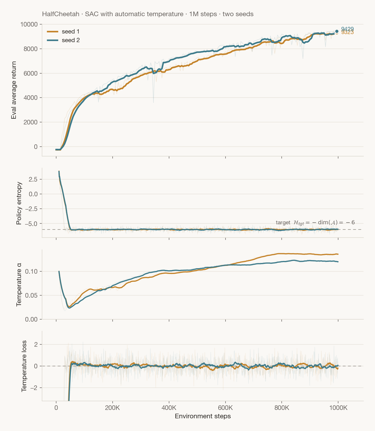
Same setup, but now $\alpha$ is the Lagrange multiplier from the section above. Dual ascent moves it to hold the constraint $\mathcal{H}(\pi) \ge \mathcal{H}_{\text{tgt}} = -\dim(\mathcal{A}) = -6$ (seeds 1 and 2). The return ends up just under 9,500 for both seeds, close to the unconstrained case, so the constraint does not seem to impact performance much. The difference is that the entropy is now controlled instead of left to drift: it reaches the target within about 50k steps and stays there for the rest of training.

HalfCheetah-v4, SAC with automatic temperature, 1M steps, two seeds. Top to bottom: eval average return, policy entropy with the target $\mathcal{H}_{\text{tgt}} = -6$, the temperature $\alpha$, and the temperature loss (y-axis clipped, the first update starts near $-22$).

The SAC agent, the actor and critic networks, and the training script can be found here.

The only thing standing between DQN and continuous actions was the max. Sampling approximates it but scales poorly. DDPG learns it, and the moment the argmax is a network, Q-learning has turned back into actor-critic: the two branches of these notes are the same loop with different policies.

The learned max amplifies the old overestimation problem, and TD3's clipped double-Q handles it by taking the pessimistic of two critics. SAC then makes the actor stochastic again and puts the exploration inside the objective as an entropy bonus, with the temperature available as a Lagrange multiplier when we want the entropy held to a target. On HalfCheetah the results are very positive.

We will go back to policy gradient next and see how we can improve it further, and hopefully show some cool results using rkt.btl!

• CS 285 Deep RL, UC Berkeley. Lecture 8: Q-Learning in Practice (PDF, Part 4 on continuous actions, Part 5 for the theory note). rail.eecs.berkeley.edu/deeprlcourse.
• Lillicrap et al., 2015. Continuous control with deep reinforcement learning (DDPG). arXiv:1509.02971.
• Fujimoto et al., 2018. Addressing Function Approximation Error in Actor-Critic Methods (TD3). arXiv:1802.09477.
• Haarnoja et al., 2018. Soft Actor-Critic (arXiv:1801.01290) and Soft Actor-Critic Algorithms and Applications (arXiv:1812.05905, the automatic temperature).
• My implementation: CS_285_Deep_RL / hw3 (DQN and SAC).