Policy Gradient - REINFORCE

Once again, these notes are more of a way to put down my thoughts on paper to solidify my understanding, and are by no means as comprehensive as the course.

This page will derive the basics necessary to understand policy gradient, by deriving its most basic algorithm: REINFORCE. We will lean on homework 2 to provide interesting results, and by the end of the page should have a solid understanding to create a bridge to actor-critic models.

This page also assumes some basic understanding of MDPs. I recommend reading Chapter 3 of Sutton's Intro to Reinforcement Learning (link) if you are not familiar with them. Or ask your favorite LLM.

REINFORCE is an on-policy (see below for meaning) algorithm that roughly consists of directly optimizing over the policy when maximizing a reward-based objective.

The objective

Let $\pi_\theta(a \mid s)$ be our policy. Running it in the environment produces a trajectory $\tau = (s_1, a_1, \ldots, s_T, a_T)$ with probability:

We want to find $\theta$ that maximizes the expected total reward:

where $r(\tau) = \sum_{t=1}^{T} r(s_t, a_t)$ is the total reward along the trajectory, a single-sample Monte Carlo estimate of $V^{\pi_\theta}(s_1)$. We can simply differentiate this expression with respect to $\theta$ and use the gradient to perform gradient ascent. This is what policy gradient effectively is.

The log trick

Pushing the gradient inside the integral:

This is exactly the score function estimator: applying that identity with $x = \tau$ and $g = r$ rewrites it as an expectation we can sample,

Now we have an expectation we can estimate from samples. The last step is to expand $\log p_\theta(\tau)$ (recall that $\log(xy) = \log(x) + \log(y)$):

Only the middle term depends on $\theta$. The initial state distribution and the dynamics drop out:

This is nice. We never need to know or model the transition dynamics. The final policy gradient is:

REINFORCE algorithm

The algorithm just turns this estimator into a loop. Sample $N$ rollouts from the current policy, average the gradient, take a step:

Why it is on-policy

The expectation is under $p_\theta(\tau)$, the current policy. As soon as we update $\theta$, the trajectories we already collected belong to the old policy. They are no longer valid samples of the new distribution, so we have to throw them out and roll out the environment again. That is what on-policy means.

The implication is sample inefficiency. We have to constantly re-roll out our policy and cannot leverage previously visited states.

If you are familiar with ML, the log term $\log \pi_\theta(a_t^{(i)} \mid s_t^{(i)})$ might look familiar to you. It is effectively the log-likelihood of action $a_t^{(i)}$ given state $s_t^{(i)}$ under our policy.

As a reminder, the gradient of the maximum-likelihood cost would look like:

The only difference is the scaling factor $r(\tau^{(i)}) = \sum_{t=1}^{T} r(s_t^{(i)}, a_t^{(i)})$ on each log gradient.

This means that each action's log gradient is scaled by the total return of its trajectory. Good action gradients get prioritized through positive multipliers, while bad ones get negatively multiplied.

We might be tempted to leave things there but will quickly encounter an issue. A single trajectory return scales every action gradient by the same scalar. We have no way to credit good moves and blame bad ones within a trajectory.

Take chess as an example. Reward is $+1$ for winning, $-1$ for losing, with games starting from random preset positions. After sampling many games, here is what we get:

• positive multipliers on actions from lucky starts and negative multipliers on unlucky starts
• negative multipliers on good moves when we blundered later
• positive multipliers on bad moves when our opponent blundered later

These issues average out with enough samples, but we might need a lot of samples to get there. This is what we call high variance.

A simple way to reduce variance is to subtract a baseline $b(s)$ from the return when scaling each log-gradient:

The intuition is simple. Without a baseline, every trajectory's return scales its action gradients in the same direction and only their magnitudes differ. Subtracting a baseline re-centers returns around zero, so good trajectories pull the gradient one way and bad ones pull it the other way. The learning signal is preserved, but the variance shrinks.

And as long as $b$ does not depend on the action, subtracting it leaves the gradient unchanged in expectation, so we pay nothing for it:

because $\mathbb{E}_\tau[\nabla_\theta \log p_\theta(\tau)] = \int \nabla_\theta p_\theta(\tau)\,d\tau = \nabla_\theta\!\int p_\theta(\tau)\,d\tau = \nabla_\theta(1) = 0$.

We will discuss specific choices of $b(s)$ further down.

You may have noticed that the scaling factor $r(\tau^{(i)}) = \sum_{t=1}^{T} r(s_t^{(i)}, a_t^{(i)})$ runs over the whole trajectory, from $t=1$ to $T$. This means an action at time $t$ is being scaled by rewards collected before it ($t' < t$), which the action could not possibly have influenced. Those past rewards are noise from the action's perspective.

One fix is to break this acausality by replacing the total return with the reward-to-go: only sum rewards from time $t$ onwards. The gradient becomes:

The good news is that this estimator is still unbiased! You can follow the proof in section 3 of the CS285 notes.

Why this helps with variance. Beyond fixing the causality issue, reward-to-go is also a variance reduction trick. The rewards we just dropped (those at $t' < t$) are uncorrelated with the action at $t$, so they contribute no signal to the gradient, but they still contribute noise. Removing them shrinks the magnitude of the multiplier without changing the underlying signal, in the same spirit as baselines.

One more standard trick is to discount future rewards by a factor $\gamma \in (0, 1]$, so the reward-to-go becomes:

Each reward counts a bit less the further into the future it is.

This helps for two reasons. Far-future rewards are noisier, since more randomness piles up over time, so down-weighting them lowers the variance. It also matches a simple intuition. The agent should care more about rewards it can reach soon, and less about far-away ones it has little control over.

$\gamma$ is just a knob: $\gamma = 1$ gives back the plain sum, smaller $\gamma$ focuses more on the near term.

If you were to compute $\nabla_\theta \log \pi_\theta(a_t^{(i)} \mid s_t^{(i)})$ explicitly, you would need an analytical (closed-form) expression for $\log \pi_\theta(a \mid s)$ and would have to differentiate it manually with respect to every parameter $\theta$, which can be cumbersome and limiting.

As we have seen before, the maximum-likelihood cost has almost the same structure as the policy gradient cost, with the difference of the scaling factor. We can just then use an MLE formulation in PyTorch with some scaling and should be able to extract the needed gradient for our iteration. Concretely, we minimize the loss:

where $\hat{A}_t^{(i)}$ is whatever scaling factor we use (for now, the reward-to-go), called advantages in the snippet below. Calling loss.backward() on this gives exactly the policy gradient estimator we derived:

def update(
    self,
    obs: np.ndarray,
    actions: np.ndarray,
    advantages: np.ndarray,
) -> dict:
    """Implements the policy gradient actor update."""
    obs = ptu.from_numpy(obs)
    actions = ptu.from_numpy(actions)
    advantages = ptu.from_numpy(advantages)

    action_distribution = self.forward(obs)
    if self.discrete:
        log_prob = action_distribution.log_prob(actions)
    else:
        #The log-probability of the full action vector is the sum of the log-probabilities of each action
        log_prob = action_distribution.log_prob(actions).sum(dim=-1)
    loss = torch.mean(-log_prob * advantages)

    self.optimizer.zero_grad()
    loss.backward()
    grad_norm = torch.nn.utils.clip_grad_norm_(self.parameters(), max_norm=float("inf"))
    self.optimizer.step()

    return {
        "Actor Loss": loss.item(),
        "Log Prob": log_prob.mean().item(),
        "Grad Norm": grad_norm.item() if isinstance(grad_norm, torch.Tensor) else float(grad_norm),
    }

The math of policy gradient does not care if the action space is discrete or continuous, but the code does. CartPole has 2 discrete actions, HalfCheetah has 6 continuous control inputs. The same training loop has to handle both.

The trick is to let the network output the parameters of a distribution and let PyTorch's Distribution API handle the rest.

For discrete actions, the network outputs one logit per possible action and the policy is the softmax over those logits:

In code, this is a Categorical distribution. Sampling returns an action index, and log_prob(a) returns a single scalar per state.

For continuous actions, the network outputs only the mean of a Gaussian. The log-std is a separate learnable parameter, shared across all states:

Two things worth pointing out:

1. The log-std is state-independent. The variance does not change based on where you are, only the mean does. This is a deliberate simplification.
2. Actions are sampled per-dimension and treated as independent. The log-probability of a vector action is the sum of per-dimension log-probabilities:

In code, this turns into action_distribution.log_prob(actions).sum(dim=-1). That .sum(dim=-1) is the only thing that differs from the discrete case.

def forward(self, obs: torch.FloatTensor) -> distributions.Distribution:
    if self.discrete:
        logits = self.logits_net(obs)
        action_distribution = distributions.Categorical(logits=logits)
    else:
        mean = self.mean_net(obs)
        std = torch.exp(self.logstd)
        action_distribution = distributions.Normal(mean, std)

    return action_distribution

action_distribution = self.forward(obs)
if self.discrete:
    log_prob = action_distribution.log_prob(actions)
else:
    #The log-probability of the full action vector is the sum of the log-probabilities of each action
    log_prob = action_distribution.log_prob(actions).sum(dim=-1)

And the actions are simply sampled as:

@torch.no_grad()
def get_action(self, obs: np.ndarray) -> np.ndarray:
    """Takes a single observation (as a numpy array) and returns a single action (as a numpy array)."""
    obs = ptu.from_numpy(obs)
    action_distribution = self.forward(obs)
    action = action_distribution.sample()

    return ptu.to_numpy(action)

We have written things abstractly with $b(s)$. Let's pick something concrete.

If we could choose any state-dependent baseline, the best one (lowest variance) is the value function:

where $Q^{\pi_\theta}$ is the true expected reward-to-go:

Subtracting it gives us the advantage: $A^{\pi_\theta} = Q^{\pi_\theta} - V^{\pi_\theta}$. In words, how much better this action is than the average action from $s_t$.

The problem is that we don't have $V^{\pi_\theta}$. The natural Monte Carlo approximation is to roll out $N$ trajectories from $s_t$ and average:

But each of those $N$ rollouts has to start from $s_t$. We would need to reset the simulator to that exact state, $N$ times, for every state we visit. This is not really advisable to do as it can get quite costly.

What we do have for free, from our normal rollouts, is one reward-to-go sample per state:

That is unbiased but very noisy ($N=1$). Used as a baseline directly, it barely helps.

The trick is to train a neural net $V_\varphi(s)$ to fit these noisy single-sample targets. Two things happen automatically:

1. Nearby states have similar values, so the network naturally averages over them.
2. We update $V_\varphi$ for $K$ steps over the same batch. The MSE loss pulls $V_\varphi$ toward the mean of the targets, contributing to the smoothing factor.

The result is an approximation of the double-sum. It will have function approximation errors, but it will keep the overall algorithm unbiased since, as previously shown, state-dependent baselines do not affect the expected value.

def update(self, obs: np.ndarray, q_values: np.ndarray) -> dict:
    obs = ptu.from_numpy(obs)
    q_values = ptu.from_numpy(q_values)

    loss = F.mse_loss(self.forward(obs).squeeze(-1), q_values)

    self.optimizer.zero_grad()
    loss.backward()
    self.optimizer.step()

    return {
        "Baseline Loss": loss.item(),
    }

One last trick that seems to always show up in practice: after computing the advantages, normalize them within each batch to have mean 0 and standard deviation 1.

where $\mu_A$ and $\sigma_A$ are the batch mean and standard deviation of the advantages, and $\epsilon$ is a small constant for numerical stability.

Interestingly this can create a bias, as the normalization depends on the specific batch we sampled. But in practice the bias is small and normalization can have a significant impact on performance as we will soon see below.

Let's recap before moving on. Our policy gradient estimator now looks like:

with the advantage

And each policy gradient iteration looks like:

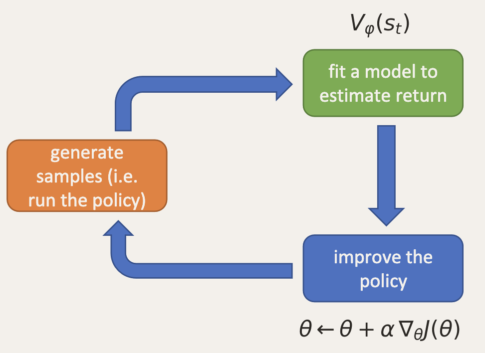
This maps onto the standard RL loop: run the policy to generate samples, fit the value model $V_\varphi(s_t)$ to estimate return, then improve the policy with a gradient step.

The policy gradient loop. Generate samples by running $\pi_\theta$, fit $V_\varphi(s_t)$ to estimate return, then improve the policy via $\theta \leftarrow \theta + \alpha\,\nabla_\theta J(\theta)$.

To see how much each variance-reduction trick actually buys us, we run REINFORCE on HalfCheetah-v4 in three configurations:

1. Basic. Reward-to-go only, no baseline, no advantage normalization.
2. Baseline. Reward-to-go minus a learned $V_\varphi$.
3. Baseline + advantage normalization. Same as above, plus per-batch advantage normalization.

All three runs share the same hyperparameters:

• Policy network: 2-layer MLP, 64 units per layer. Gaussian policy with learned std for continuous actions.
• Value network (when used): same shape as the policy, scalar output.
• Optimizer: Adam with $\text{lr} = 0.01$ for both networks.
• Discount: $\gamma = 0.95$.
• Batch size: 5000 environment steps per iteration.
• Eval batch: 3000 environment steps every iteration.
• Critic updates: 5 MSE gradient steps per policy update (when the baseline is used).
• Iterations: 100. About 500k environment steps per run.

The exact CLI commands are the ones the HW2 spec suggests:

# Basic (reward-to-go, no baseline)
uv run src/scripts/run.py --env_name HalfCheetah-v4 -n 100 -b 5000 -eb 3000 -rtg \
  --discount 0.95 -lr 0.01 --exp_name cheetah

# With baseline
uv run src/scripts/run.py --env_name HalfCheetah-v4 -n 100 -b 5000 -eb 3000 -rtg \
  --discount 0.95 -lr 0.01 --use_baseline -blr 0.01 -bgs 5 --exp_name cheetah_baseline

# With baseline + advantage normalization
uv run src/scripts/run.py --env_name HalfCheetah-v4 -n 100 -b 5000 -eb 3000 -rtg \
  --discount 0.95 -lr 0.01 --use_baseline -blr 0.01 -bgs 5 -na --exp_name cheetah_baseline_na

Each curve is the best of about five runs at different seeds, since policy gradient is sensitive to initial conditions (you can see the gradient sometimes going in the wrong direction at the start).

HalfCheetah-v4. Eval average return over 500k environment steps. Basic peaks at −240. Adding a baseline brings the peak to 352. Adding advantage normalization on top jumps the peak to 739.

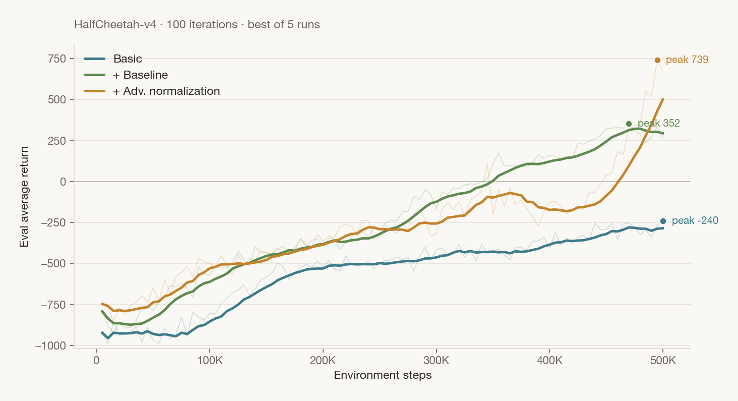
The basic estimator, reward-to-go only, climbs steadily from −1000 toward 0 but never makes it. The single-sample $\hat{Q}$ is just too noisy for the policy to find consistent improvements.

Adding the baseline helps significantly. Subtracting $V_\varphi(s_t)$ lets the policy reach consistently positive returns and peak above 350 over the same number of environment steps.

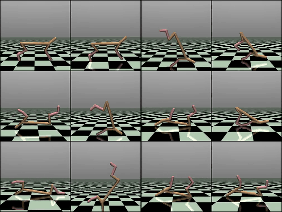
Normalization has a big impact on performance. The peak jumps to 739, and looking at the gifs below the cheetah is actually running rather than break dancing.

Basic
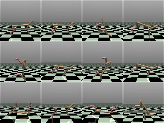
peak −240

Baseline
peak 352

Baseline + adv. norm.
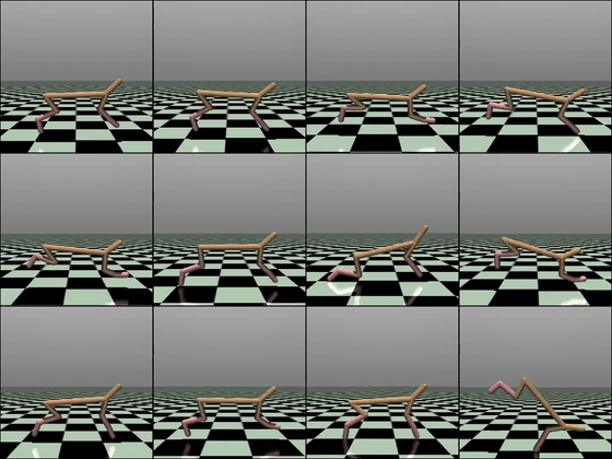
peak 739

It makes sense that normalizing the advantage helps reduce gradient variance: as mentioned before, it prevents the policy from taking overly large steps. This matters because advantage magnitudes tend to grow as the policy improves and rewards get larger.

And so we are done with our first dive into policy gradient. The derivation is pretty straightforward once you see the log-derivative trick. All the variance reduction ideas (baseline, causality, discounting, and normalization) are intuitive to understand and show real impact during implementation.

Recall that we currently rely on a MC estimate $\hat{Q}_t^{(i)} = \sum_{t'=t}^{T} \gamma^{t'-t}\, r(s_{t'}^{(i)}, a_{t'}^{(i)})$ for the Q value inside the advantage. We will see next how we can improve on this using bootstrapping, which will bring us to our first actor-critic formulation.

• CS 285 Deep RL, UC Berkeley. Lectures 4–6: RL basics, Policy gradients, Actor-critic. Spring 2026. rail.eecs.berkeley.edu/deeprlcourse.
• CS 285 Deep RL, UC Berkeley. HW2: Policy Gradients. PDF.
• Sutton & Barto. Reinforcement Learning: An Introduction, Chapter 13. link. Especially §13.4 (REINFORCE with baseline) and §13.5 (Actor-critic methods).
• Schulman et al. High-Dimensional Continuous Control Using Generalized Advantage Estimation. ICLR 2016. arXiv:1506.02438.

If you made it to the bottom of this one too, try running the secret shell ./hobbit.sh in the terminal of the homepage.