
Advanced DQN - Completing the Rainbow
This continues the Q-Learning notes, which left us with a working DQN. In practice we can add more features to improve performance. The full version is often called Rainbow, after the DeepMind paper that combined them. This page goes through each extra feature to complete the rainbow. This part is outside the CS285 syllabus.
Where we left off
On the previous page we started from the naive algorithm and found it would not train:
and fixed it with three components that together make plain DQN:
- Target network. Build the target from a frozen copy $Q_{\bar\varphi}$, refreshed every $N$ steps, so the labels stop moving under the regression.
- $n$-step returns. Carry $n$ real rewards before bootstrapping, so reward propagates $n$ states per update instead of one.
- Double Q-learning. Let the online net pick the next action and the target net score it, which cancels most of the $\max$ overestimation bias.
In practice, the Rainbow paper (Hessel et al., 2018, DeepMind) found that combining more features increases performance. There is a total of 6 stackable features in that paper and we are already familiar with two of them (double Q-learning and multi-step returns). On this page we will discuss in detail the remaining four.
- Dueling networks. Split the head into a state value $V(s)$ and a per-action advantage $A(s,a)$.
- Prioritized experience replay. Sample transitions by TD error instead of uniformly.
- Distributional RL (C51). Predict the whole distribution of the return, not just its mean.
- Noisy nets. Replace $\epsilon$-greedy with learnable noise on the weights.
Dueling networks
This trick is for performance only and is a way to effectively increase the sample efficiency of DQN.
In practice there are often states where the action barely matters. Either the control authority at that state is low, or whatever you press, the outlook is roughly the same (like if the goal is far away, for instance). So when you decompose the $Q$ value as
$$Q(s,a) = V(s) + A(s,a),$$it is often the case that $V(s)$ dominates and the advantage is just a small correction on top.
The idea of dueling networks is to mirror this decomposition in the critic. Instead of the critic network outputting $|\mathcal{A}|$ $Q(s,a)$ values, we change the output to have two heads: a scalar $V(s)$ and a vector $A(s,a)$, and sum them as a final step.
Why the split helps
I was confused at first why this split would help, since the $Q$ value (what we really care about) is left unchanged. This has to do with the underlying neural network and how the gradient backpropagates.
Look at what a single transition $(s, a)$ teaches a plain DQN. The loss keeps only the taken action's $Q$-value:
qa_values = self.critic.forward(obs)
q_values = qa_values[batch_idx, action.long()]
loss = self.critic_loss(q_values, target_values)
The middle line selects, for each $(s, a)$ transition in the batch, only the column of the action that was taken. The loss effectively disregards all other outputs, so their gradient is 0. If action 2 of 4 was taken, only output 2's weights get updated; actions 0, 1 and 3 get nothing from this sample, and their values move only indirectly, through the shared hidden layers.
  transition (s, a),  a = 2  (of 4 actions)

    Q(s, 0)   gradient 0
    Q(s, 1)   gradient 0
    Q(s, 2)   gradient nonzero   <-- only the taken action
    Q(s, 3)   gradient 0
This means each output only learns from its own action's visits. An update to $Q(s, a_1)$ might not change the output for $Q(s, a_2)$ the next time it is queried. It is as if the shared value $V(s)$ were repeated inside every output and had to be relearned each time. It takes on the order of $|\mathcal{A}|$ updates, over different actions, for the network to move the $Q$-values of all of them.
The dueling head removes this duplication. Since $Q(s,a) = V(s) + A(s,a)$, the same $V(s)$ feeds every action's $Q$-value:
$$\frac{\partial Q(s,a)}{\partial V(s)} = 1 \quad \text{for every action } a.$$Every transition sends a full gradient into $V(s)$, whichever action it used. If a state is visited $N$ times, a plain head gives each action's output only about $N / |\mathcal{A}|$ updates, while the dueling $V(s)$ gets all $N$, so the value converges roughly $|\mathcal{A}|$ times sooner and one action's update moves the $Q$-values of the rest. This compounds through bootstrapping: the TD target for other transitions reads $Q(s')$, so getting the updated $Q$ sooner feeds better targets back into the rest of the updates. Overall the trick helps most when $|\mathcal{A}|$ is large.
Making the split identifiable
There is one problem to fix before this works. Written as $Q = V + A$, the split is not unique: add any constant $c$ to $V$ and subtract it from every $A(s,a)$, and $Q$ is unchanged,
$$\big(V(s) + c\big) + \big(A(s,a) - c\big) = V(s) + A(s,a).$$The loss only ever sees $Q$, so nothing forces $V$ to be the value and $A$ to be the advantage. The network could assign any values to them. We say the decomposition is unidentifiable, and we need another constraint, otherwise the separation we are attempting would be in vain.
The fix is to remove the free direction by centering the advantage. Subtract its mean over actions before adding:
$$Q(s,a) = V(s) + \Big( A(s,a) - \frac{1}{|\mathcal{A}|} \sum_{a'} A(s,a') \Big).$$To see why this pins the split down, sum both sides over the $|\mathcal{A}|$ actions. The centered term sums to zero by construction, so
$$\sum_a Q(s,a) = |\mathcal{A}|\, V(s) + \underbrace{\sum_a A(s,a) - \sum_a A(s,a)}_{0} \;\;\Longrightarrow\;\; V(s) = \frac{1}{|\mathcal{A}|} \sum_a Q(s,a).$$$V$ is now forced to be the mean of the $Q$-values across actions, and the advantage head the deviation from that mean. The free constant is gone, the two heads are identifiable, and $Q$ itself is unchanged.
In code
The critic keeps the same hidden stack, then two linear heads instead of one, recombined with the mean-centered advantage:
class DuelingDQNCritic(nn.Module):
    def __init__(self, observation_shape, num_actions, n_layers, size):
        super().__init__()
        input_size = int(np.prod(observation_shape))
        # Shared torso: same hidden stack as DQNCritic, but stopping at the last
        # hidden activation (size features) instead of projecting to num_actions.
        self.torso = ptu.build_mlp(
            input_size=input_size,
            output_size=size,
            n_layers=max(n_layers - 1, 0),
            size=size,
            output_activation="tanh",
        )
        self.value_head = nn.Linear(size, 1)
        self.advantage_head = nn.Linear(size, num_actions)

    def forward(self, obs):
        # Flatten observations if needed
        if obs.ndim > 2:
            obs = obs.reshape(obs.shape[0], -1)
        features = self.torso(obs)
        value = self.value_head(features)  # (batch_size, 1)
        advantage = self.advantage_head(features)  # (batch_size, num_actions)
        return value + advantage - advantage.mean(dim=1, keepdim=True)
Next up: prioritized experience replay.
Distributional RL (C51)
The return distribution behind $Q$ can be multi-modal, and solely operating on its mean $Q$ can throw away a lot of information. C51 breaks that return distribution into a histogram per action instead of the single number $Q$. We still use the mean when selecting the action, but the Bellman update now propagates the whole distribution instead of a single mean, so the learned values should be more accurate.
Predicting a distribution instead of a number
We first fix a grid of possible return values $z_i$, called the atoms. Take $N$ points evenly spaced on some range $[V_{\min}, V_{\max}]$,
$$z_i = V_{\min} + i\, \Delta z, \qquad \Delta z = \frac{V_{\max} - V_{\min}}{N - 1}, \qquad i = 0, \dots, N-1.$$The critic then outputs, for each action, a probability $p_i(s,a)$ on each atom (a softmax over $N$ logits); write $p(s,a)$ for the whole vector of these probabilities. The return $Z(s,a)$ is a random variable, and its distribution is a categorical: a probability spread over a fixed, finite set of values, here the atoms,
$$Z(s,a) \;\sim\; \sum_{i} p_i(s,a)\, \delta_{z_i}, \qquad \sum_i p_i(s,a) = 1.$$Each $\delta_{z_i}$ is a point mass (a Dirac delta) at the atom $z_i$.
The original paper settled on $51$ atoms with a categorical distribution, which led to the name C51. Action selection is left unchanged, as we still operate on the mean,
$$Q(s,a) = \mathbb{E}[Z(s,a)] = \sum_i z_i\, p_i(s,a),$$and act greedily on that.
The distributional Bellman update
Everything in this section is about building the training target. Plain DQN turns each transition $(s, a, r, s')$ into a scalar target $y = r + \gamma\, Q(s', a^*)$ and pushes $Q(s,a)$ toward it. C51 does the same thing one level up: from the transition, build a target distribution $m$ on the fixed atoms, then push the predicted distribution of $Z(s,a)$ toward it. For our distribution the Bellman equation can be written as,
$$Z(s,a) \;\overset{D}{=}\; r + \gamma\, Z(s', a^*), \qquad a^* = \arg\max_{a'} Q(s', a'),$$where $\overset{D}{=}$ means the two sides have the same distribution.
We can build the target distribution $m$ in 3 steps.
Step 1: get the next-state distribution. Query the target network at $s'$. It gives probabilities $p_i(s', a^*)$ on the atoms $z_i$ (e.g. the return from $s'$ is $z_i$ with probability $p_i$). This is similar to $Q(s', a^*)$ in the vanilla scalar target case.
Step 2: apply reward and discount. If the return from $s'$ is $z_i$, then the return from $s$ is $r + \gamma z_i$. So each atom moves,
$$z_i \;\longmapsto\; \operatorname{clamp}\big(r + \gamma z_i,\; V_{\min},\; V_{\max}\big).$$The clamping is to enforce the values to remain in the fixed grid range. The probabilities of each $z_i$ have not changed with this step, but note that the shifted $z_i$ might now not fall exactly on the fixed grid. So we have the correct distribution, but it is effectively "shifted", and we need to re-express (shift) it onto our fixed grid, as the loss has to compare the target to the prediction atom by atom.
Step 3: project back onto the grid. The projection is done by splitting the shifted value's probability between its neighboring grid atoms based on its distance. This can be shown to keep the total mass to $1$:
  support:   ... 8 ─── 9 ─── 10 ─── 11 ─── 12 ...   (Δz = 1)

  a shifted atom lands at 10.3 carrying probability 0.2
      atom 10  gets  0.2 · (11 - 10.3) = 0.14
      atom 11  gets  0.2 · (10.3 - 10) = 0.06
Summing the contributions of all the shifted values gives the target distribution $m$ on the fixed support.
The loss is a cross-entropy
Prediction $p(s,a)$ and target $m$ now live on the same atoms, so we can easily compare them. C51 minimizes the cross-entropy between them,
$$\mathcal{L} = - \sum_i m_i \, \log p_i(s,a),$$which is the KL divergence from the target to the prediction up to a constant. This replaces the scalar MSE from plain DQN. Everything else is untouched.
In code
class DistributionalDQNCritic(nn.Module):
    def __init__(self, observation_shape, num_actions, n_layers, size,
                 num_atoms=51, v_min=-10.0, v_max=10.0):
        super().__init__()
        self.num_actions = num_actions
        self.num_atoms = num_atoms
        self.v_min = v_min
        self.v_max = v_max
        self.net = ptu.build_mlp(
            input_size=int(np.prod(observation_shape)),
            output_size=num_actions * num_atoms,
            n_layers=n_layers,
            size=size,
        )
        # Fixed atom locations z_0 ... z_{num_atoms-1}, shared across states and
        # actions. Registered as a buffer so it moves with .to(device) and is
        # saved in the state dict.
        self.register_buffer("support", torch.linspace(v_min, v_max, num_atoms))

    def dist(self, obs):
        if obs.ndim > 2:
            obs = obs.reshape(obs.shape[0], -1)
        logits = self.net(obs).reshape(-1, self.num_actions, self.num_atoms)
        return torch.softmax(logits, dim=-1)

    def forward(self, obs):
        probs = self.dist(obs)  # (batch_size, num_actions, num_atoms)
        return torch.sum(probs * self.support, dim=-1)
with torch.no_grad():
    # Greedy next action from the expected Q-values. Under double-Q the
    # online net picks the action; the target net always supplies the
    # distribution.
    if self.use_double_q:
        next_action = torch.argmax(self.critic.forward(next_obs), dim=1)
    else:
        next_action = torch.argmax(self.target_critic.forward(next_obs), dim=1)

    next_probs = self.target_critic.dist(next_obs)  # (B, A, num_atoms)
    next_probs = next_probs[batch_idx, next_action.long()]  # (B, num_atoms)

    # Shift every atom by the Bellman update, then clamp back onto the
    # support. reward/done broadcast over the atom axis.
    reward = reward.unsqueeze(1)  # (B, 1)
    not_done = (1 - done.float()).unsqueeze(1)  # (B, 1)
    Tz = reward + self.discount * not_done * support.unsqueeze(0)  # (B, atoms)
    Tz = Tz.clamp(v_min, v_max)

    # Categorical projection: spread each shifted atom's probability onto
    # the two nearest fixed atoms.
    b = (Tz - v_min) / delta_z  # (B, atoms), in [0, num_atoms - 1]
    lower = b.floor().long()
    upper = b.ceil().long()

    # When b lands exactly on an atom, lower == upper and both weights are
    # zero; nudge the pair apart so that atom keeps its full mass.
    lower[(upper > 0) & (lower == upper)] -= 1
    upper[(lower < num_atoms - 1) & (lower == upper)] += 1

    target_dist = torch.zeros_like(next_probs)  # (B, num_atoms)
    target_dist.scatter_add_(1, lower, next_probs * (upper.float() - b))
    target_dist.scatter_add_(1, upper, next_probs * (b - lower.float()))

log_probs = torch.log(self.critic.dist(obs) + 1e-8)  # (B, A, num_atoms)
log_probs = log_probs[batch_idx, action.long()]  # (B, num_atoms)
loss = -(target_dist * log_probs).sum(dim=1).mean()
Noisy nets
Plain DQN explores with $\epsilon$-greedy: with probability $\epsilon$ it takes a random action, otherwise the greedy one. The randomness is the same in every state, and $\epsilon$ follows a schedule set by hand. Noisy nets add learnable noise to the weights instead. The noise level is a parameter on each weight, trained along with everything else, so the network is in charge of its own exploration: how much to explore and when to wind it down.
Noise on the weights
We can simply take any linear layer $y = W x + b$ and make its parameters noisy. Each weight becomes a learned mean plus a learned scale times fresh random noise,
$$y = (\mu_W + \sigma_W \odot \varepsilon_W)\, x + (\mu_b + \sigma_b \odot \varepsilon_b),$$where $\mu$ and $\sigma$ are learned parameters, $\varepsilon$ is noise resampled each step, and $\odot$ is elementwise. $\mu$ is the weight, $\sigma$ is how much noise to add to it. A layer like this is a NoisyLinear. The noisy critic is the same MLP with each linear layer replaced by one.
If each parameter had its own independent noise $\varepsilon$, we would need $\text{in} \times \text{out}$ random numbers per layer per step. Instead we use factorized noise: draw one noise vector for the inputs and one for the outputs, then take their outer product,
$$\varepsilon_W[i,j] = f(\varepsilon^{\text{out}}_i)\, f(\varepsilon^{\text{in}}_j), \qquad f(x) = \operatorname{sign}(x)\sqrt{|x|},$$with $\varepsilon^{\text{in}}$ and $\varepsilon^{\text{out}}$ unit Gaussians of length $\text{in}$ and $\text{out}$. That is $\text{in} + \text{out}$ random numbers instead of $\text{in} \times \text{out}$, and the bias reuses $\varepsilon^{\text{out}}$.
Why this explores, and why it anneals
The weight noise shifts the $Q$-values on every forward pass. Sometimes the shift is enough to make a different action the largest, and the agent tries it instead of the current greedy one. That is the exploration. It is not a uniform random action like $\epsilon$-greedy: the shift on each $Q$-value is scaled by the learned $\sigma$ of the weights feeding it, so the ones with larger $\sigma$ move more.
$\sigma$ is trained by the same TD gradient as the weights. On average the noise only adds error to the fit, so the gradient pushes $\sigma$ down or leaves it flat, never up. Where the critic already fits the target well, $\sigma$ is driven toward zero, since the noise is pure cost there. Where the fit is still poor it has not been driven down yet, so exploration lingers where the network is unsure and fades where it has settled, with no schedule set by hand. And since the perturbation depends on the input, the noise is state dependent.
In code
A NoisyLinear keeps $\mu$ and $\sigma$ as parameters and the noise as buffers. reset_noise draws a fresh perturbation, and forward uses $\mu + \sigma \odot \varepsilon$ while training but just $\mu$ at eval time, so evaluation is deterministic:
class NoisyLinear(nn.Module):
    def __init__(self, in_features, out_features, sigma_0=0.5):
        super().__init__()
        self.in_features = in_features
        self.out_features = out_features
        self.sigma_0 = sigma_0

        # Learned mean and noise-scale for the weights and biases.
        self.weight_mu = nn.Parameter(torch.empty(out_features, in_features))
        self.weight_sigma = nn.Parameter(torch.empty(out_features, in_features))
        self.bias_mu = nn.Parameter(torch.empty(out_features))
        self.bias_sigma = nn.Parameter(torch.empty(out_features))

        # Noise samples: not trained, resampled by reset_noise(). Registered as
        # buffers so they move with .to(device) and are saved in the state dict.
        self.register_buffer("weight_epsilon", torch.empty(out_features, in_features))
        self.register_buffer("bias_epsilon", torch.empty(out_features))

        self.reset_parameters()
        self.reset_noise()

    def reset_parameters(self):
        # mu ~ U[-1/sqrt(p), 1/sqrt(p)] and sigma = sigma_0 / sqrt(p), with
        # p = in_features, following the factorized-noise setup in the paper.
        bound = 1.0 / np.sqrt(self.in_features)
        self.weight_mu.data.uniform_(-bound, bound)
        self.bias_mu.data.uniform_(-bound, bound)
        self.weight_sigma.data.fill_(self.sigma_0 * bound)
        self.bias_sigma.data.fill_(self.sigma_0 * bound)

    def _scale_noise(self, size):
        x = torch.randn(size, device=self.weight_mu.device)
        return x.sign() * x.abs().sqrt()

    def reset_noise(self):
        eps_in = self._scale_noise(self.in_features)
        eps_out = self._scale_noise(self.out_features)
        # Factorized outer product for the weight noise; the bias reuses eps_out.
        self.weight_epsilon.copy_(torch.outer(eps_out, eps_in))
        self.bias_epsilon.copy_(eps_out)

    def forward(self, x):
        if self.training:
            weight = self.weight_mu + self.weight_sigma * self.weight_epsilon
            bias = self.bias_mu + self.bias_sigma * self.bias_epsilon
        else:
            weight = self.weight_mu
            bias = self.bias_mu
        return nn.functional.linear(x, weight, bias)
Plugging it into DQN needs almost nothing else. We resample the noise once per update for both the online and target critics, and again before each action. Since the network now explores on its own, $\epsilon$-greedy is turned off (the exploration schedule is set to $0$). The loss and the rest of the agent are unchanged.
Prioritized replay
Uniform replay draws every stored transition with equal probability. But not every transition teaches the same amount. One the critic already predicts well has little left to correct, while one with a large temporal-difference error is exactly where the critic is still wrong. Prioritized replay samples the high-error transitions more often, so the updates spend their time where the error is.
Sampling by TD error
Give each transition a priority $p_i = |\delta_i| + \epsilon$, where $\delta_i$ is its last TD error and $\epsilon$ is a small constant so no priority reaches zero and drops out for good. Sample transition $i$ with probability
$$P(i) = \frac{p_i^\alpha}{\sum_k p_k^\alpha}.$$The exponent $\alpha$ sets how strong the prioritization is: $\alpha = 0$ is uniform replay, $\alpha = 1$ samples in direct proportion to the priority. A new transition has no TD error yet, so it goes in at the largest priority seen so far. That way it is sampled at least once, and its priority is corrected from a real error after that.
Correcting the bias
Sampling the high-error transitions more often changes the distribution the updates average over, which biases the fit toward those transitions. Importance sampling undoes it: weight transition $i$'s update by
$$w_i = \left(\frac{1}{N\, P(i)}\right)^{\beta},$$with $N$ the number of stored transitions and $P(i)$ its sampling probability from above. Concretely, $w_i$ scales that sample's squared error in the critic loss,
$$L = \frac{1}{B}\sum_i w_i\, \delta_i^2,$$with $B$ the batch size and $\delta_i$ the sample's TD error from above, in place of the plain mean over the batch. A transition we drew too often has a large $P(i)$, so its weight is small, which cancels the oversampling. The exponent $\beta$ sets how much of the bias we correct: at $\beta = 1$ it is fully corrected. It generally starts at a low value and is annealed up to $1$ over training, since the bias matters most late, when the fit is close and the remaining error is small. The weights in a batch are divided by their maximum, so they only ever scale an update down, which keeps the step sizes stable.
In code
The buffer stores $p_i^\alpha$ in a sum-tree, a binary tree whose leaves hold the priorities and whose internal nodes hold the sum of their two children, so the root is the total priority:
           9            root = total priority
          / \
         4   5          internal = sum of children
        / \ / \
       3  1 2  3        leaves    = p_i^alpha
To sample, draw a value $u$ uniformly in $[0, \text{total})$ and walk down from the root: at each node go left if $u$ is below the left child's sum, otherwise subtract that sum and go right. You land on a leaf with probability proportional to its priority, in $O(\log N)$. A priority update overwrites one leaf and adds the change along the path back to the root, also $O(\log N)$. sample returns the importance weights alongside the batch, and update_priorities writes back the fresh errors after the step:
    def sample(self, batch_size, beta=None):
        beta = self.beta if beta is None else beta
        data_idcs = self.tree.sample(batch_size)
        # Guard against a leaf past the filled region (possible only before the
        # buffer has seen batch_size inserts).
        data_idcs = np.clip(data_idcs, 0, self.size - 1)

        probs = self.tree.leaf(data_idcs) / self.tree.total
        n = min(self.size, self.max_size)
        weights = (n * probs) ** (-beta)
        weights = weights / weights.max()

        return {
            "observations": self.observations[data_idcs],
            "actions": self.actions[data_idcs],
            "rewards": self.rewards[data_idcs],
            "next_observations": self.next_observations[data_idcs],
            "dones": self.dones[data_idcs],
            "indices": data_idcs,
            "weights": weights.astype(np.float32),
        }

    def update_priorities(self, data_idcs: np.ndarray, priorities: np.ndarray):
        priorities = np.abs(priorities) + self.eps
        self.max_priority = max(self.max_priority, float(priorities.max()))
        self.tree.update(np.asarray(data_idcs), priorities ** self.alpha)
The training loop scales each sample's squared error by its weight before averaging, the $L$ from above, then hands the batch's fresh errors back to the buffer so their priorities update. Nothing else in the agent changes.
Results
Each component above was first written against the small vector critic, then extended to the Atari convolutional path so they can run together on pixels. The combined agent for MsPacman is a single conv critic that switches each Rainbow head on or off through flags. The whole rewrite is on GitHub: the AtariCritic that combines every head, and the full-Rainbow MsPacman config.
I ran a leave-one-out ablation on MsPacman. The configs are:
- full Rainbow, every feature on
- Rainbow with one feature removed: double-Q, dueling, C51, noisy nets, or prioritized replay (5 runs)
- Rainbow with both noisy nets and C51 removed
- plain DQN, every feature off
That is 8 configs, each for 1M environment steps, over 3 seeds, so 24 runs. Each curve below is the mean over its 3 seeds, with the raw eval trace faint behind the smoothed line.
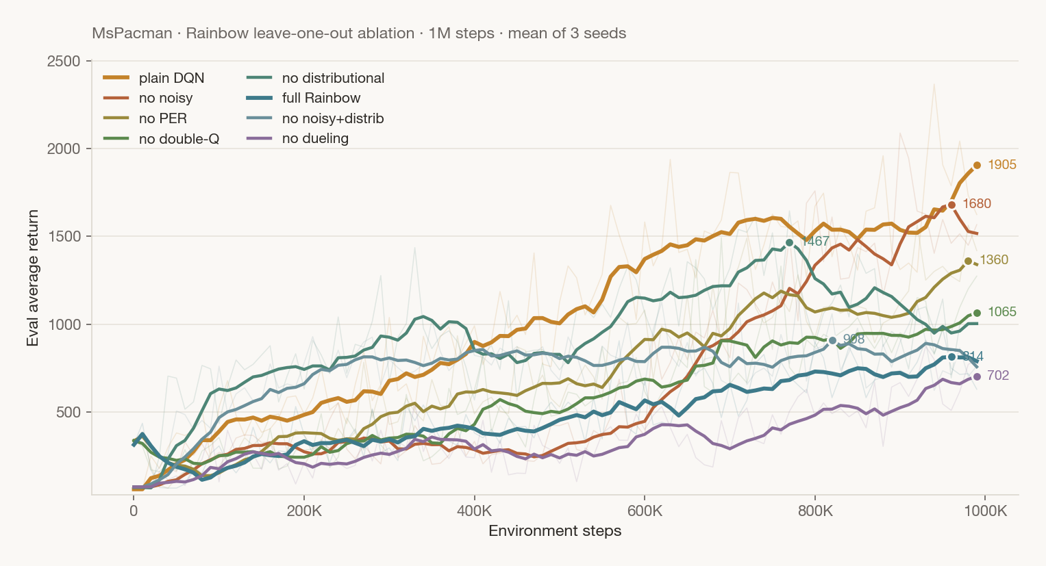
The results are mixed, which was surprising at first. Plain DQN, with every extra feature off, has the highest return here, and full Rainbow is near the bottom. Removing most components helped rather than hurt. Dueling is the exception: removing it from Rainbow made the return a bit lower, so it seems to be the only feature that helped on this game.
The table ranks the configs by their final return, measured as the mean of each run's last five evals, averaged over the 3 seeds. This is less noisy than a single final point. The last column is the single best eval any seed reached.
| config | final return (mean ± sd) | best single eval |
|---|---|---|
| plain DQN (all off) | 1819 ± 318 | 4710 |
| Rainbow − noisy nets | 1517 ± 89 | 4570 |
| Rainbow − PER | 1365 ± 134 | 4140 |
| Rainbow − double-Q | 1099 ± 346 | 3910 |
| Rainbow − C51 | 991 ± 245 | 4520 |
| full Rainbow | 757 ± 241 | 4080 |
| Rainbow − noisy − C51 | 755 ± 194 | 3910 |
| Rainbow − dueling | 648 ± 118 | 2040 |
I think Rainbow is probably over-engineered for this setup. The features were tuned together on the full Atari suite at 50 to 200M frames, and at 1M steps on a single game they seem to hurt more than help. Noisy nets hurt the most: with C51 on, removing them raised the return from 757 to 1517. So the components interact, and their effects do not add up independently.
C51 also needs a value range $[v_{\min}, v_{\max}]$ for its atoms. I set $v_{\min} = 0$, since MsPacman rewards are never negative, and $v_{\max} = 2600$, chosen empirically from the returns and the $0.99$ discount as headroom for the discounted value of a good run.